4-Node
Structural Shell
SHELL181 Element Description
SHELL181 is suitable for analyzing thin to moderately-thick shell structures. It is a four-node element with six degrees of freedom at each node: translations in the x, y, and z directions, and rotations about the x, y, and z-axes. (If the membrane option is used, the element has translational degrees of freedom only). The degenerate triangular option should only be used as filler elements in mesh generation.
SHELL181 is well-suited for linear, large rotation, and/or large strain nonlinear applications. Change in shell thickness is accounted for in nonlinear analyses. In the element domain, both full and reduced integration schemes are supported. SHELL181 accounts for follower (load stiffness) effects of distributed pressures.
SHELL181 can be used for layered applications for modeling composite shells or sandwich construction. The accuracy in modeling composite shells is governed by the first-order shear-deformation theory (usually referred to as Mindlin-Reissner shell theory).
The element formulation is based on logarithmic strain and true stress measures. The element kinematics allow for finite membrane strains (stretching). However, the curvature changes within a time increment are assumed to be small.
See SHELL181 for more details about this element.
SHELL181 Input Data
The following figure shows the geometry, node locations, and the element coordinate system for this element. The element is defined by shell section information and by four nodes (I, J, K, and L).
Figure 181.1: SHELL181 Geometry
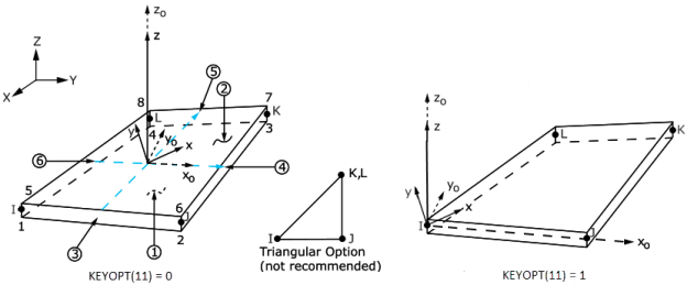
x0 = Element x axis if element orientation (ESYS) is not specified.
x = Element x axis if element orientation is specified.
Single-Layer Definition
To define the thickness (and other information), use section definition, as follows:
| SECTYPE,,SHELL |
SECDATA,THICKNESS, ... |
A single-layer shell section definition provides flexible options. For example, you can specify the number of integration points used and the material orientation.
Multilayer Definition
The shell section commands allow for layered shell definition. Options are available for specifying the thickness, material, orientation, and number of integration points through the thickness of the layers.
You can designate the number of integration points (1, 3, 5, 7, or 9) located through the thickness of each layer when using section input. When only one, the point is always located midway between the top and bottom surfaces. If three or more points, two points are located on the top and bottom surfaces respectively and the remaining points are distributed equal distance between the two points. The default number of integration points for each layer is three; however, when a single layer is defined and plasticity is present, the number of integration points is changed to a minimum of five during solution.
The following additional capabilities are available when defining shell layers:
SHELL181 accepts the preintegrated shell section type (SECTYPE,,GENS).
When the element is associated with the GENS section type, thickness or material definitions are not required.
You can use the function tool to define thickness as a function of global/local coordinates or node numbers (SECFUNCTION).
You can specify offsets (SECOFFSET).
Other Input
When KEYOPT(11) = 0, the default orientation for this element has the S1 (shell surface coordinate) axis aligned with the first parametric direction of the element at the center of the element, which connects the midsides of edges LI and JK and is shown as xo in Figure 181.1: SHELL181 Geometry. In the most general case, the axis can be defined as:

where:

|
| {x}I, {x}J, {x}K, {x}L = global nodal coordinates |
If edges IJ and KL are parallel (rectangular or trapezoidal elements), the default orientation is the same as described in Coordinate Systems (the first surface direction is aligned with the IJ side). For elements with nonparallel edges IJ and JK, the default orientation represents the stress state better because the element uses a single point of quadrature (by default) in the element domain.
With KEYOPT(11) = 1, the default element coordinate x0 axis is directed from node I to node J. The z0 axis is normal to the shell surface, and the y0 axis is perpendicular to the x0 and z0 axes.
The default element orientation can be rotated by angle θ (in degrees) for the layer (SECDATA). For an element, you can specify a single value of orientation in the plane of the element. Layer-wise orientation is supported.
You can also define element orientation via the ESYS command. See Coordinate Systems.
The element supports degeneration into a triangular form; however, use of the triangular form is not recommended, except when used as mesh filler elements or with the membrane option (KEYOPT(1) = 1). The triangle form is generally more robust when using the membrane option with large deflections.
To evaluate stresses and strains on exterior surfaces, use KEYOPT(1) = 2. When used as overlaid elements on the faces of 3-D elements, this option is similar to the surface stress option (described in the Mechanical APDL Theory Reference), but is more general and applicable to nonlinear analysis. The element used with this option does not provide any stiffness, mass, or load contributions. This option should only be used in single-layer shells. Irrespective of other settings, SHELL181 provides stress and strain output at the center of the layer.
SHELL181 uses a penalty method to relate the independent rotational degrees of freedom about the normal (to the shell surface) with the in-plane components of displacements. The program chooses an appropriate penalty stiffness by default. A drill stiffness factor can be specified via the SECCONTROL command.
Element loads are described in Nodal Loading. Pressures can be input as surface loads on the element faces as shown by the circled numbers on Figure 181.1: SHELL181 Geometry. Positive pressures act into the element. Because shell edge pressures are input on a per-unit-length basis, per-unit-area quantities must be multiplied by the shell thickness.
Temperatures can be input as element body loads at the corners of the outside faces of the element and at the corners of the interfaces between layers. The first corner temperature T1 defaults to TUNIF. If all other temperatures are unspecified, they default to T1. If KEYOPT(1) = 0 and if exactly NL+1 temperatures are input, one temperature is used for the four bottom corners of each layer, and the last temperature is used for the four top corner temperatures of the top layer. If KEYOPT(1) = 1 and if exactly NL temperatures are input, one temperature is used for the four corners of each layer. That is, T1 is used for T1, T2, T3, and T4; T2 (as input) is used for T5, T6, T7, and T8, etc. For any other input pattern, unspecified temperatures default to TUNIF.
Using KEYOPT(3), SHELL181 supports uniform reduced integration and full integration with incompatible modes. By default, this element uses the uniform reduced integration for performance reasons in nonlinear applications.
Using reduced integration with hourglass control creates some usage restrictions, although minimal. For example, to capture the in-plane bending of a cantilever or a stiffener (see Figure 181.2: SHELL181 Typical Bending Applications), a number of elements through the thickness direction is necessary. The performance gains achieved by using uniform reduced integration are significant enough to offset the need to use more elements. In relatively well-refined meshes, hourglassing issues are largely irrelevant.
When the reduced integration option is used, you can check the accuracy of the solution by comparing the total energy (SENE label in ETABLE) and the artificial energy (AENE label in ETABLE) introduced by hourglass control. If the ratio of artificial energy to total energy is less than 5%, the solution is generally acceptable. The total energy and artificial energy can also be monitored by using OUTPR,VENG in the solution phase.
Bilinear elements, when fully integrated, are too stiff in in-plane bending.SHELL181 uses the method of incompatible modes to enhance the accuracy in bending-dominated problems. This approach is also called "extra shapes" or "bubble" modes approach. SHELL181 uses the formulation that ensures satisfaction of the patch test (J. C. Simo and F. Armero, "Geometrically nonlinear enhanced strain mixed methods and the method of incompatible modes," IJNME, Vol. 33, pp. 1413-1449, 1992).
When including incompatible modes in the analysis, you must use full integration. KEYOPT(3) = 2 implies the inclusion of incompatible modes and the use of full (2x2) quadrature.
SHELL181, with KEYOPT(3) = 2 specified, does not have any spurious energy mechanisms. This specific form of SHELL181 is highly accurate, even with coarse meshes. Use KEYOPT(3) = 2 if you encounter any hourglass-related difficulties with the default options. KEYOPT(3) = 2 is also necessary if the mesh is coarse and in-plane bending of the elements dominate the response. We recommend this option with all layered applications.
KEYOPT(3) = 2 imposes the fewest usage restrictions. You can always choose this option. However, you can improve element performance by choosing the best option for your problem. Consider the problems illustrated in Figure 181.2: SHELL181 Typical Bending Applications


The cantilever beam and the beam cross-section to be modeled with shells are typical examples of in-plane bending-dominated problems. The use of KEYOPT(3) = 2 is the most effective choice in these circumstances. Reduced integration would require refined meshes. For example, reduced integration for the cantilever beam problem requires four elements through the thickness, whereas the full integration with incompatible modes only requires one element through the thickness.
For the stiffened shell, the most effective choice is to use KEYOPT(3) = 0 for the shell and KEYOPT(3) = 2 for the stiffener.
When KEYOPT(3) = 0 is specified, SHELL181 uses an hourglass control method for membrane and bending modes. By default, SHELL181 calculates the hourglass parameters for both metal and hyperelastic applications. To specify the hourglass stiffness scaling factors, use the SECCONTROL command.
When KEYOPT(5) = 1, the element uses an advanced formulation that incorporates initial curvature effects. The calculation for effective shell curvature change accounts for both shell-membrane and thickness strains. The formulation generally offers improved accuracy in curved shell structure simulations, especially when thickness strain is significant or the material anisotropy in the thickness direction cannot be ignored, or in thick shell structures with unbalanced laminate construction or with shell offsets. The initial curvature of each element is calculated from the nodal shell normals. The shell normal at each node is obtained by averaging the shell normals from the surrounding SHELL181 elements. A coarse or highly distorted shell mesh can lead to significant error in the recovered element curvature; therefore, this option should be used with a smooth, adequately refined mesh only. To ensure proper representation of the original mesh, a nodal normal is replaced by the element shell normal in the curvature calculation if the subtended angle between these two is greater than 25 degrees.
When KEYOPT(5) = 2, a simplified curved-shell formulation is adopted. Unlike the advanced curved-shell formulation (KEYOPT(5) =1), the curvature effects in the shell offset handling are ignored. The simplified formulation generally leads to more robust nonlinear convergence.
SHELL181 includes the linear effects of transverse shear deformation. An assumed shear strain formulation of Bathe-Dvorkin is used to alleviate shear locking. The transverse shear stiffness of the element is a 2x2 matrix as shown below:

Transverse shear effects are not included in the normal material constitutive modeling for this element.
To define transverse shear stiffness values, issue the SECCONTROL command.
Transverse shear-correction factors k are calculated once at the start of the analysis for each section. The material properties used to evaluate the transverse shear correction factors are at the current reference temperature during solution. User-field variables and frequency are all set to zero when evaluating the material properties used to calculate the transverse shear correction factors.
For a single-layer shell with isotropic material, default transverse shear stiffnesses are:

In the above matrix, shear-correction factor k = 5/6, G = shear modulus, and h = thickness of the shell.
SHELL181 can be associated with linear elastic, elastoplastic, creep, or hyperelastic material properties. Only isotropic, anisotropic, and orthotropic linear elastic properties can be input for elasticity. The von Mises isotropic hardening plasticity models can be invoked with BISO (bilinear isotropic hardening), and NLISO (nonlinear isotropic hardening) options. The kinematic hardening plasticity models can be invoked with BKIN (bilinear kinematic hardening), and CHABOCHE (nonlinear kinematic hardening). Invoking plasticity assumes that the elastic properties are isotropic (that is, if orthotropic elasticity is used with plasticity, the program assumes the isotropic elastic modulus = EX and Poisson's ratio = NUXY).
Hyperelastic material properties (2, 3, 5, or 9 parameter Mooney-Rivlin material model, Neo-Hookean model, Polynomial form model, Arruda-Boyce model, and user-defined model) can be used with this element. Poisson's ratio is used to specify the compressibility of the material. If less than 0, Poisson's ratio is set to 0; if greater than or equal to 0.5, Poisson's ratio is set to 0.5 (fully incompressible).
Both isotropic and orthotropic thermal expansion coefficients can be input using MP,ALPX. When used with hyperelasticity, isotropic expansion is assumed.
Use the TREF command to specify the global value of reference temperature. If MP,REFT is defined for the material number of the element, it is used for the element instead of the value from the TREF command. But if MP,REFT is defined for the material number of the layer, it is used instead of either the global or element value.
With reduced integration and hourglass control (KEYOPT(3) = 0), low frequency spurious modes can appear if the mass matrix employed is not consistent with the quadrature rule. SHELL181 uses a projection scheme that effectively filters out the inertia contributions to the hourglass modes of the element. To be effective, a consistent mass matrix must be used. We recommend setting LUMPM,OFF for a modal analysis using this element type. The lumped mass option can, however, be used with the full integration options (KEYOPT(3) = 2).
KEYOPT(8) = 2 stores midsurface results in the results file for single or multi-layer shell elements. If you use SHELL,MID, you will see these calculated values, rather than the average of the TOP and BOTTOM results. You should use this option to access these correct midsurface results (membrane results) for those analyses where averaging TOP and BOTTOM results is inappropriate; examples include midsurface stresses and strains with nonlinear material behavior, and midsurface results after mode combinations that involve squaring operations such as in spectrum analyses.
KEYOPT(9) = 1 reads initial thickness data from a user subroutine.
KEYOPT(10) = 1 outputs normal stress component Sz, where z is shell
normal direction. The element uses a plane-stress formulation that always leads to zero thickness
normal stress. With KEYOPT(10) = 1, Sz is independently recovered during the element solution
output from the applied pressure load. The pressure must be applied directly to the shell, and
not via surface elements (SURFnnn).
You can apply an initial stress state to this element via the INISTATE command. For more information, see Initial State in the Mechanical APDL Advanced Analysis Guide.
The effects of pressure load stiffness are automatically included for this element. If an unsymmetric matrix is needed for pressure load stiffness effects, use NROPT,UNSYM.
A summary of the element input is given in "SHELL181 Input Summary". A general description of element input is given in Element Input.
SHELL181 Input Summary
- Nodes
I, J, K, L
- Degrees of Freedom
UX, UY, UZ, ROTX, ROTY, ROTZ if KEYOPT(1) = 0
UX, UY, UZ if KEYOPT(1) = 1
- Material Properties
TB command: See Element Support for Material Models for this element. MP command: EX, EY, EZ, (PRXY, PRYZ, PRXZ, or NUXY, NUYZ, NUXZ), ALPX, ALPY, ALPZ (or CTEX, CTEY, CTEZ or THSX, THSY, THSZ), DENS, GXY, GYZ, GXZ, ALPD Specify BETD, ALPD, and DMPR for the element (all layers) by issuing the MAT command to assign the material property set. REFT can be specified once for the element, or it can be assigned on a per-layer basis. See the discussion in "SHELL181 Input Summary" for more information. - Surface Loads
- Pressures --
face 1 (I-J-K-L) (bottom, in +N direction), face 2 (I-J-K-L) (top, in -N direction), face 3 (J-I), face 4 (K-J), face 5 (L-K), face 6 (I-L) - Equivalent source surface flag --
MXWF (input on the SF command)
- Body Loads
- Temperatures --
For KEYOPT(1) = 0 (Bending and membrane stiffness):
T1, T2, T3, T4 (at bottom of layer 1), T5, T6, T7, T8 (between layers 1-2); similarly for between next layers, ending with temperatures at top of layer NL(4*(NL+1) maximum). Hence, for one-layer elements, 8 temperatures are used.
For KEYOPT(1) = 1 (Membrane stiffness only):
T1, T2, T3, T4 for layer 1, T5, T6, T7, T8 for layer 2, similarly for all layers (4*NL maximum). Hence, for one-layer elements, 4 temperatures are used.
- Special Features
Birth and death Coriolis effect Element technology autoselect Initial state Large deflection Large strain Linear perturbation Nonlinear stabilization Section definition for layered shells and preintegrated general shell sections for input of homogeneous section stiffnesses Stress stiffening - KEYOPT(1)
Element stiffness:
- 0 --
Bending and membrane stiffness (default)
- 1 --
Membrane stiffness only
- 2 --
Stress/strain evaluation only
- KEYOPT(3)
Integration option:
- 0 --
Reduced integration with hourglass control (default)
- 2 --
Full integration with incompatible modes
- KEYOPT(5)
Curved shell formulation:
- 0 --
Standard shell formulation (default)
- 1 --
Advanced curved-shell formation
- 2 --
Simplified curved-shell formation
- KEYOPT(8)
Specify layer data storage:
- 0 --
For multi-layer elements, store data for bottom of bottom layer and top of top layer. For single-layer elements, store data for TOP and BOTTOM. (Default)
- 1 --
Store data for TOP and BOTTOM, for all layers (multi-layer elements)
Note: Volume of data may be excessive.
- 2 --
Store data for TOP, BOTTOM, and MID for all layers; applies to single- and multi-layer elements
- KEYOPT(9)
User thickness option:
- 0 --
No user subroutine to provide initial thickness (default)
- 1 --
Read initial thickness data from user-defined subroutine
UTHICKSee the Guide to User-Programmable Features in the Mechanical APDL Programmer's Reference for user-defined subroutines
- KEYOPT(10)
Thickness normal stress (Sz) output option:
- 0 --
Sz not modified (default, Sz = 0)
- 1 --
Recover and output Sz from applied pressure load
- KEYOPT(11)
Default element x axis (x0) orientation:
- 0 --
First parametric direction at the element centroid (default)
- 1 --
Pointing from element node I to element node J
SHELL181 Output Data
The solution output associated with the element is in two forms:
Nodal displacements included in the overall nodal solution
Additional element output as shown in Table 181.1: SHELL181 Element Output Definitions
Several items are illustrated in Figure 181.3: SHELL181 Stress Output.
KEYOPT(8) controls the amount of data output to the results file for processing with the LAYER command. Interlaminar shear stress is available as SYZ and SXZ evaluated at the layer interfaces. KEYOPT(8) must be set to either 1 or 2 to output these stresses in POST1. A general description of solution output is given in Solution Output. See the Basic Analysis Guide for ways to review results.
The element stress resultants (N11, M11, Q13, etc.) are parallel to the element coordinate system, as are the membrane strains and curvatures of the element. Such generalized strains are available through the SMISC option at the element centroid only. The transverse shear forces Q13, Q23 are available only in resultant form: that is, use SMISC,7 (or 8). Likewise, the transverse shear strains, γ13 and γ23, are constant through the thickness and are only available as SMISC items (SMISC,15 and SMISC,16, respectively).
The program calculates moments (M11, M22, M12) with respect
to the shell reference plane. By default, ANSYS adopts the shell midplane
as the reference plane. To offset the reference plane to any other
specified location, issue the SECOFFSET command.
When there is a nonzero offset (L) from the reference plane to the
midplane, moments with respect to the midplane ( ) can be
recovered from stress resultants with respect to the reference plane
as follows:
) can be
recovered from stress resultants with respect to the reference plane
as follows:

SHELL181 does not support extensive basic element printout. POST1 provides more comprehensive output processing tools; therefore, ANSYS suggests using the OUTRES command to ensure that the required results are stored in the database.
Figure 181.3: SHELL181 Stress Output

x0 = Element x axis if element orientation (ESYS) is not specified. (See KEYOPT(11).) x = Element x axis if element orientation is specified.
The Element Output Definitions table uses the following notation:
A colon (:) in the Name column indicates that the item can be accessed by the Component Name method (ETABLE, ESOL). The O column indicates the availability of the items in the file Jobname.OUT. The R column indicates the availability of the items in the results file.
In either the O or R columns, “Y” indicates that the item is always available, a number refers to a table footnote that describes when the item is conditionally available, and “-” indicates that the item is not available.
Table 181.1: SHELL181 Element Output Definitions
| Name | Definition | O | R |
|---|---|---|---|
| EL | Element number and name | Y | Y |
| NODES | Nodes - I, J, K, L | - | Y |
| MAT | Material number | - | Y |
| THICK | Average thickness | - | Y |
| VOLU: | Volume | - | Y |
| XC, YC, ZC | Location where results are reported | - | 4 |
| PRES | Pressures P1 at nodes I, J, K, L; P2 at I, J, K, L; P3 at J,I; P4 at K,J; P5 at L,K; P6 at I,L | - | Y |
| TEMP | T1, T2, T3, T4 at bottom of layer 1, T5, T6, T7, T8 between layers 1-2, similarly for between next layers, ending with temperatures at top of layer NL(4*(NL+1) maximum) | - | Y |
| LOC | TOP, MID, BOT, or integration point location | - | 1 |
| S:X, Y, Z, XY, YZ, XZ | Stresses | 3 | 1 |
| S:1, 2, 3 | Principal stresses | - | 1 |
| S:INT | Stress intensity | - | 1 |
| S:EQV | Equivalent stress | - | 1 |
| EPEL:X, Y, Z, XY | Elastic strains | 3 | 1 |
| EPEL:EQV | Equivalent elastic strains [7] | - | 1 |
| EPTH:X, Y, Z, XY | Thermal strains | 3 | 1 |
| EPTH:EQV | Equivalent thermal strains [7] | - | 1 |
| EPPL:X, Y, Z, XY | Average plastic strains | 3 | 2 |
| EPPL:EQV | Equivalent plastic strains [7] | - | 2 |
| EPCR:X, Y, Z, XY | Average creep strains | 3 | 2 |
| EPCR:EQV | Equivalent creep strains [7] | - | 2 |
| EPTO:X, Y, Z, XY | Total mechanical strains (EPEL + EPPL + EPCR) | 3 | - |
| EPTO:EQV | Total equivalent mechanical strains (EPEL + EPPL + EPCR) | - | - |
| NL:SEPL | Plastic yield stress | - | 2 |
| NL:EPEQ | Accumulated equivalent plastic strain | - | 2 |
| NL:CREQ | Accumulated equivalent creep strain | - | 2 |
| NL:SRAT | Plastic yielding (1 = actively yielding, 0 = not yielding) | - | 2 |
| NL:PLWK | Plastic work/volume | - | 2 |
| NL:HPRES | Hydrostatic pressure | - | 2 |
| SEND:ELASTIC, PLASTIC, CREEP, ENTO | Strain energy densities | - | 2 |
| N11, N22, N12 | In-plane forces (per unit length) | - | Y |
| M11, M22, M12 | Out-of-plane moments (per unit length) | - | 8 |
| Q13, Q23 | Transverse shear forces (per unit length) | - | 8 |
| ε11, ε22, ε12 | Membrane strains | - | Y |
| k11, k22, k12 | Curvatures | - | 8 |
| γ13, γ23 | Transverse shear strains | - | 8 |
| LOCI:X, Y, Z | Integration point locations | - | 5 |
| SVAR:1, 2, ... , N | State variables | - | 6 |
| ILSXZ | SXZ interlaminar shear stress | - | Y |
| ILSYZ | SYZ interlaminar shear stress | - | Y |
| ILSUM | Magnitude of the interlaminar shear stress vector | - | Y |
| ILANG | Angle of interlaminar shear stress vector (measured from the element x axis toward the element y axis in degrees) | - | Y |
| Sm: 11, 22, 12 | Membrane stresses | - | Y |
| Sb: 11, 22, 12 | Bending stresses | - | Y |
| Sp: 11, 22, 12 | Peak stresses | - | Y |
| St: 13, 23 | Averaged transverse shear stresses | - | Y |
The following stress solution repeats for top, middle, and bottom surfaces.
Nonlinear solution output for top, middle, and bottom surfaces, if the element has a nonlinear material, or if large-deflection effects are enabled (NLGEOM,ON) for SEND.
Stresses, total strains, plastic strains, elastic strains, creep strains, and thermal strains in the element coordinate system are available for output (at all section points through thickness). If layers are in use, the results are in the layer coordinate system.
Available only at centroid as a *GET item.
Available only if OUTRES,LOCI is used.
Available only if the
UserMatsubroutine and TB,STATE command are used.The equivalent strains use an effective Poisson's ratio: for elastic and thermal this value is set by the user (MP,PRXY); for plastic and creep this value is set at 0.5.
Not available if the membrane element option is used (KEYOPT(1) = 1).
Table 181.2: SHELL181 Item and Sequence Numbers lists output available through ETABLE using the Sequence Number method. See Creating an Element Table and The Item and Sequence Number Table in this reference for more information. The following notation is used in Table 181.2: SHELL181 Item and Sequence Numbers:
- Name
output quantity as defined in the Table 181.1: SHELL181 Element Output Definitions
- Item
predetermined Item label for ETABLE
- E
sequence number for single-valued or constant element data
- I,J,K,L
sequence number for data at nodes I, J, K, L
Table 181.2: SHELL181 Item and Sequence Numbers
| Output Quantity Name | ETABLE and ESOL Command Input | |||||
|---|---|---|---|---|---|---|
| Item | E | I | J | K | L | |
| N11 | SMISC | 1 | - | - | - | - |
| N22 | SMISC | 2 | - | - | - | - |
| N12 | SMISC | 3 | - | - | - | - |
| M11 | SMISC | 4 | - | - | - | - |
| M22 | SMISC | 5 | - | - | - | - |
| M12 | SMISC | 6 | - | - | - | - |
| Q13 | SMISC | 7 | - | - | - | - |
| Q23 | SMISC | 8 | - | - | - | - |
| ε11 | SMISC | 9 | - | - | - | - |
| ε22 | SMISC | 10 | - | - | - | - |
| ε12 | SMISC | 11 | - | - | - | - |
| k11 | SMISC | 12 | - | - | - | - |
| k22 | SMISC | 13 | - | - | - | - |
| k12 | SMISC | 14 | - | - | - | - |
| γ13 | SMISC | 15 | - | - | - | - |
| γ23 | SMISC | 16 | - | - | - | - |
| THICK | SMISC | 17 | - | - | - | - |
| P1 | SMISC | - | 18 | 19 | 20 | 21 |
| P2 | SMISC | - | 22 | 23 | 24 | 25 |
| P3 | SMISC | - | 27 | 26 | - | - |
| P4 | SMISC | - | - | 29 | 28 | - |
| P5 | SMISC | - | - | - | 31 | 30 |
| P6 | SMISC | - | 32 | - | - | 33 |
| Sm: 11 | SMISC | 34 | - | - | - | - |
| Sm: 22 | SMISC | 35 | - | - | - | - |
| Sm: 12 | SMISC | 36 | - | - | - | - |
| Sb: 11 | SMISC | 37 | - | - | - | - |
| Sb: 22 | SMISC | 38 | - | - | - | - |
| Sb: 12 | SMISC | 39 | - | - | - | - |
| Sp: 11 (at shell bottom) | SMISC | 40 | - | - | - | - |
| Sp: 22 (at shell bottom) | SMISC | 41 | - | - | - | - |
| Sp: 12 (at shell bottom) | SMISC | 42 | - | - | - | - |
| Sp: 11 (at shell top) | SMISC | 43 | - | - | - | - |
| Sp: 22 (at shell top) | SMISC | 44 | - | - | - | - |
| Sp: 12 (at shell top) | SMISC | 45 | - | - | - | - |
| St: 13 | SMISC | 46 | - | - | - | - |
| St: 23 | SMISC | 47 | - | - | - | - |
SHELL181 Assumptions and Restrictions
ANSYS, Inc. recommends against using this element in triangular form, except as a filler element. Avoid triangular form especially in areas with high stress gradients.
Zero-area elements are not allowed. (Zero-area elements occur most often whenever the elements are numbered improperly.)
Zero thickness elements or elements tapering down to a zero thickness at any corner are not allowed (but zero thickness layers are allowed).
If multiple load steps are used, the number of layers cannot change between load steps.
When the element is associated with preintegrated shell sections (SECTYPE,,GENS), additional restrictions apply. For more information, see Considerations for Using Preintegrated Shell Sections in the Mechanical APDL Structural Analysis Guide.
If reduced integration is used (KEYOPT(3) = 0) SHELL181 ignores rotary inertia effects when an unbalanced laminate construction is used, and all inertial effects are assumed to be in the nodal plane (that is, an unbalanced laminate construction and offsets have no effect on the mass properties of the element).
For most composite analyses, ANSYS, Inc. recommends setting KEYOPT(3) = 2 (necessary to capture the stress gradients).
No slippage is assumed between the element layers. Shear deflections are included in the element; however, normals to the center plane before deformation are assumed to remain straight after deformation.
Transverse shear stiffness of the shell section is estimated by an energy equivalence procedure (of the generalized section forces and strains vs. the material point stresses and strains). The accuracy of this calculation may be adversely affected if the ratio of material stiffnesses (Young's moduli) between adjacent layers is very high.
The calculation of interlaminar shear stresses is based on simplifying assumptions of unidirectional, uncoupled bending in each direction. If accurate edge interlaminar shear stresses are required, shell-to-solid submodeling should be used.
The section definition permits use of hyperelastic material models and elastoplastic material models in laminate definition; however, the accuracy of the solution is primarily governed by fundamental assumptions of shell theory. The applicability of shell theory in such cases is best understood by using a comparable solid model.
The layer orientation angle has no effect if the material of the layer is hyperelastic.
Before using this element in a simulation containing curved thick shell structures with unbalanced laminate construction or shell offsets, validate the usage via full 3-D modeling with a solid element in a simpler representative model. The element may underestimate the curved thick shell stiffness, particularly when the offset is large and the structure is under torsional load. Consider using curved-shell formulation (KEYOPT(5) = 1).
The through-thickness stress, SZ, is always zero.
This element works best with the full Newton-Raphson solution scheme (NROPT,FULL,,ON).
Stress stiffening is always included in geometrically nonlinear analyses (NLGEOM,ON). Prestress effects can be activated by the PSTRES command.
In a nonlinear analysis, the solution process terminates if the thickness at any integration point that was defined with a nonzero thickness vanishes (within a small numerical tolerance).
If a shell section has only one layer and the number of section integration points is equal to one, or if KEYOPT(1) = 1, then the shell has no bending stiffness, a condition that can result in solver and convergence problems.
SHELL181 Product Restrictions
When used in the product(s) listed below, the stated product-specific restrictions apply to this element in addition to the general assumptions and restrictions given in the previous section.
ANSYS Mechanical Pro
Birth and death is not available.
Initial state is not available.
Linear perturbation is not available.
Section definition for layered shells in not available.
ANSYS Mechanical Premium
Birth and death is not available.