2-D Hydrostatic
Fluid
HSFLD241 Element Description
HSFLD241 is used to model fluids that are fully enclosed by solids (containing vessels). The hydrostatic fluid element is well suited for calculating fluid volume and pressure for coupled problems involving fluid-solid interaction. The pressure in the fluid volume is assumed to be uniform (no pressure gradients), so sloshing effects cannot be included. Temperature effects and compressibility may be included, but fluid viscosity cannot be included.
Hydrostatic fluid elements are overlaid on the faces of 2-D solid elements enclosing the fluid volume. See HSFLD241 in the Mechanical APDL Theory Reference for more details about this element. See HSFLD242 for a 3-D version of this element.
HSFLD241 Input Data
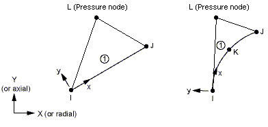
The geometry, node locations, and the coordinate system for this element are shown in Figure 241.1: HSFLD241 Geometry. The hydrostatic fluid element is defined by three or four nodes. Nodes I, J and K on the surface (face 1) are shared with the solid element and have two degrees of freedom at each node: translation in x and y directions. Node K is not used if the underlying solid element does not have a midside node. For the case of a degenerate solid element sharing the collapsed face with the hydrostatic fluid element, the surface nodes of the hydrostatic fluid element will be coincident. Node L is a pressure node with a hydrostatic pressure degree of freedom. Hydrostatic fluid elements can be generated automatically using the ESURF command.
The pressure node (L) can be located anywhere in the fluid volume, except when the fluid volume has symmetry boundaries; in this case the pressure node must be located on the symmetry line or on the intersection point of multiple symmetry lines. The pressure node is automatically moved to the centroid of the fluid volume if there are no displacement degree-of-freedom constraints specified. To keep the pressure node on a symmetry line, you must specify symmetry boundary conditions at this node. (The displacement degrees of freedom at the pressure node do not have any displacement solution associated with them. They are only available for applying displacement degree of freedom constraints.) The pressure node is shared by all the hydrostatic fluid elements used to define the fluid volume. It is also used to apply temperature loads, fluid mass flow rate, or hydrostatic pressure degree-of-freedom constraints for the fluid.
You can define a hydrostatic fluid element without an underlying solid element in situations where the underlying solid has a discontinuity. In this case, the surface nodes (I and J) of the hydrostatic fluid element must be shared with adjacent solid elements, or the displacement degrees of freedom at the surface nodes should be constrained. For example, the gap between the cylinder and piston in a cylinder-piston assembly with fluid may be bridged with a hydrostatic fluid element by sharing one of its surface nodes (I) with a solid element on the cylinder and its other surface node (J) with a solid element on the piston (see Example Model Using Hydrostatic Fluid Elements in the Structural Analysis Guide).
You can define material properties for hydrostatic fluid elements using MP or TB commands. All hydrostatic fluid elements sharing a pressure node must use the same material property definition and must have the same real constant values (THK and PREF).
You can input element thickness and reference pressure (must
be specified for compressible gas defined via TB command with Lab = FLUID and TBOPT = GAS) as real constants THK and PREF. The THK
value is used to calculate element volume.
You can define the initial state of the hydrostatic fluid by
defining initial pressure (input via the IC command
with Lab = HDSP) at the pressure node.
Specify the reference temperature by using the TREF command or the MP,REFT command. For compressible
gas (defined via the TB command with Lab = FLUID and TBOPT =
GAS), the initial pressure and the reference pressure (input as real
constant PREF) are added internally to get the total initial pressure
for the Ideal Gas Law. Internal force corresponding to initial pressure
is calculated internally and applied over the first load step.
You can prescribe uniform pressure for the fluid as a hydrostatic
pressure degree-of-freedom constraint at the pressure node (input
on D command with Lab = HDSP). The change in hydrostatic pressure value is assumed to
occur as a result of the addition or removal of fluid mass to or from
the containing vessel. Applying a hydrostatic pressure degree-of-freedom
constraint is equivalent to applying a surface load on the underlying
solid element surface. Element loads are described in Nodal Loading. You can apply fluid mass flow rate as a load
on the pressure node (input via F command with Lab = DVOL); a positive value indicates fluid mass
flowing into the containing vessel. You can also input fluid temperature
as an element body load at the pressure node (input via BF command with Lab = TEMP). The nodal temperature
defaults to TUNIF.
You can model fluid flow between two fluid volumes in two containing vessels by using FLUID116 coupled thermal-fluid pipe elements to connect the pressure nodes of the two fluid volumes (using only one FLUID116 element is recommended). You can also model fluid flow through an orifice between a fluid volume and the atmosphere by connecting one node of a FLUID116 element with the HSFLD241 pressure node; the other node of the FLUID116 element represents environmental pressure. For either of these scenarios, you must activate the PRES degree of freedom (KEYOPT(1) = 1) on the pressure node of the hydrostatic fluid elements, and you must set KEYOPT(1) = 3 on the FLUID116 element.
KEYOPT(1) defines degrees of freedom for the hydrostatic fluid element:
| Use KEYOPT(1) = 0 (default) to activate UX and UY degrees of freedom on the surface nodes (I, J, K) and HDSP degree of freedom on the pressure node (L). |
| Use KEYOPT(1) = 1 to activate UX, and UY degrees of freedom on surface nodes (I, J, K) and HDSP and PRES degrees of freedom on the pressure node (L). You must activate the PRES degree of freedom if the pressure node of the hydrostatic fluid element is shared with a coupled thermal-fluid pipe (FLUID116) element to model fluid flow. |
KEYOPT(3) defines the hydrostatic fluid element behavior:
| Use KEYOPT(3) = 0 (default) to model planar behavior. The choice of plane stress or plane strain is made automatically based on the attached solid element. |
| Use KEYOPT(3) = 1 to model 2-D axisymmetric behavior. |
KEYOPT(5) specifies how mass is computed for the hydrostatic fluid element:
| Use KEYOPT(5) = 0 (default) to ignore the mass contribution from the fluid element. However, you can attach MASS21 elements to the nodes of the underlying 2-D solid elements to account for the fluid mass. |
| Use KEYOPT(5) = 1 to distribute the fluid element mass to the surface nodes (I, J, K) based on the volume of the fluid element. No mass is added to the surface nodes if the volume of the fluid element becomes negative. |
| Use KEYOPT(5) = 2 to distribute the fluid element mass to the surface nodes (I, J, K) based on the ratio of element surface area (area of face 1) to the total fluid surface area. |
KEYOPT(6) defines the hydrostatic fluid element compressibility:
Use KEYOPT(6) = 0 (default) to model the hydrostatic fluid
element as compressible. You need to define a fluid material property
(use the TB command with Lab = FLUID) to relate changes in fluid pressure to fluid volume. |
| Use KEYOPT(6) = 1 or 2 to model the hydrostatic fluid element as incompressible. The fluid volume is kept constant, even as the solid enclosing the fluid undergoes large deformations. The fluid volume, however, can change when fluid mass is added to or taken out of the containing vessel; this is achieved by applying a fluid mass flow rate or by prescribing a non-zero hydrostatic pressure degree-of-freedom constraint at the pressure node. The fluid volume can also change when a temperature load is applied at the pressure node for a fluid with a non-zero coefficient of thermal expansion. When KEYOPT(6) = 1, the change in volume is accommodated by a change in fluid mass (mass flows into or out of the cavity). When KEYOPT(6) = 2, the change in volume is accommodated by a change in fluid density such that fluid mass is held constant. |
You can define contact and target surfaces on the attached 2-D solid elements to model self-contact between walls of the containing vessel after the fluid has been removed. Note that contact should not cause a single fluid region to be separated into two since the pressure-volume calculations are performed assuming a single cavity.
For more information on using hydrostatic fluid elements to model fluids enclosed by solids, see Modeling Hydrostatic Fluids in the Structural Analysis Guide.
"HSFLD241 Input Summary" contains a summary of the element input. See Element Input in this document for a general description of element input.
HSFLD241 Input Summary
- Nodes
I, J, K, L
- Degrees of Freedom
UX, UY for surface nodes (I, J, K)
HDSP and PRES for pressure node (L)
- Real Constants
THK - Thickness
PREF - Reference pressure for compressible gas defined via TB command with
Lab= FLUID andTBOPT= GAS- Material Properties
MP command: ALPX, DENS, ALPD
- Surface Loads
None
- Body Loads
- Temperatures --
T(L)
- Special Features
Large deflection Linear perturbation Nonlinearity - KEYOPT(1)
Degrees of freedom:
- 0 --
UX and UY degrees of freedom at surface nodes, HDSP degree of freedom at pressure node (default)
- 1 --
UX and UY degrees of freedom at surface nodes, HDSP and PRES degrees of freedom at pressure node
- KEYOPT(3)
Element behavior:
- 0 --
Planar (default)
- 1 --
Axisymmetric
- KEYOPT(5)
Fluid mass:
- 0 --
No fluid mass (default)
- 1 --
Fluid mass calculated based on the volume of the fluid element
- 2 --
Fluid mass calculated based on the surface area of the fluid element
- KEYOPT(6)
Fluid compressibility:
- 0 --
Compressible (default)
- 1 --
Incompressible
- 2 --
Incompressible, but allows change in density under thermal expansion
HSFLD241 Output Data
The solution output associated with the element is in two forms:
Nodal degrees of freedom included in the overall nodal solution
Additional element output as shown in Table 241.1: HSFLD241 Element Output Definitions
A general description of solution output is given in Solution Output. See the Basic Analysis Guide for ways to view results.
The Element Output Definitions table uses the following notation:
A colon (:) in the Name column indicates that the item can be accessed by the Component Name method (ETABLE, ESOL). The O column indicates the availability of the items in the file Jobname.OUT. The R column indicates the availability of the items in the results file.
In either the O or R columns, “Y” indicates that the item is always available, a number refers to a table footnote that describes when the item is conditionally available, and “-” indicates that the item is not available.
Table 241.1: HSFLD241 Element Output Definitions
| Name | Definition | O | R |
|---|---|---|---|
| EL | Element Number | Y | Y |
| NODES | Nodes - I, J, K, L | Y | Y |
| MAT | Material number | Y | Y |
| AREA | Element surface area (face 1) | Y | Y |
| VOLU | Element volume | Y | Y |
| XC, YC | Location on the surface (face 1) where results are reported | Y | 1 |
| DENSITY | Fluid density | Y | Y |
| TEMP | Temperature at nodes: T(I), T(J), T(K), T(L) | Y | Y |
| TVOL | Total volume of the fluid in the containing vessel | 2 | 2 |
| TMAS | Total mass of the fluid in the containing vessel | 3 | 3 |
| MFLO | Fluid mass flow rate | 4 | 4 |
| TVOLO | Total original volume of the fluid in the containing vessel | 2 | 2 |
Available only at centroid as a *GET item.
Elements that share a pressure node have the same TVOL and TVOLO output value.
Elements that share a pressure node have the same TMAS output value.
Elements that share a pressure node have the same MFLO output value.
Table 241.2: HSFLD241 Item and Sequence Numbers lists output available through the ETABLE command using the Sequence Number method. See The General Postprocessor (POST1) in the Basic Analysis Guide and The Item and Sequence Number Table in this reference for more information. The following notation is used in Table 241.2: HSFLD241 Item and Sequence Numbers:
- Name
output quantity as defined in Table 241.1: HSFLD241 Element Output Definitions
- Item
predetermined Item label for ETABLE command
- E
sequence number for single-valued or constant element data
HSFLD241 Assumptions and Restrictions
The fluid volume has no free surface; it is completely enclosed by the solid (containing vessel).
The fluid volume has uniform pressure, temperature, and density without any gradients.
All elements used to define a fluid volume share a pressure node with a hydrostatic pressure degree of freedom.
The pressure node can be located anywhere within the fluid volume; it is automatically moved to the centroid of the fluid volume if there are no displacement degree-of-freedom constraints specified. However, if the fluid volume is bounded by one or more symmetry lines, the pressure node must be on the symmetry line or intersecting corner of multiple symmetry lines, and it must have symmetry boundary conditions.
The fluid may be modeled as incompressible or compressible without any viscosity.
The PRES degree of freedom must be active (KEYOPT(1) = 1) on the pressure node of the hydrostatic fluid element to model fluid flow with FLUID116 coupled thermal-fluid pipe elements. In this case, the PRES (pressure) and HDSP (hydrostatic pressure) degrees of freedom are made to be the same at the pressure node.
Inertial effects such as sloshing cannot be included, but fluid mass can be added to the surface nodes (I, J, K) shared with the underlying 2-D solid by using KEYOPT(5).
This element can be used in linear and nonlinear static and transient analyses and modal analyses.