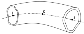
3-D 3-Node Elbow
ELBOW290 Element Description
The ELBOW290 element is suitable for analyzing tubular structures with thin to moderately thick walls. The element accounts for cross-section distortion, which can be commonly observed in curved pipe structures under loading.
ELBOW290 is a quadratic (three-node) pipe element in 3-D. The element has six degrees of freedom at each node (the translations in the x, y, and z directions and rotations about the x, y, and z directions). The element is well-suited for linear, large rotation, and/or large strain nonlinear applications. Change in pipe thickness is accounted for in geometrically nonlinear analyses. The element accounts for follower (load stiffness) effects of distributed pressures.
The element can be used in layered applications for modeling laminated composite pipes. The accuracy in modeling composite pipes is governed by the first-order shear-deformation theory (generally referred to as Mindlin-Reissner shell theory).
The element supports the pipe cross-section defined via SECTYPE, SECDATA, and SECOFFSET commands.
ELBOW290 is available in two forms:
Structural Elbow -- See "ELBOW290 Structural Elbow Description".
Generalized Structural Tube -- "ELBOW290 Generalized Tube Description"
For more detailed information about this element, see ELBOW290 - 3-D 3-Node Elbow in the Mechanical APDL Theory Reference.
ELBOW290 Structural Elbow Description
The ELBOW290 Structural Elbow is suitable for modeling pipe bends (elbows) or straight pipes that may undergo large deformation. The pipes being modeled must have round cross-sections. Pipe wall thickness and outside diameter cannot vary within each element

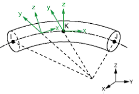
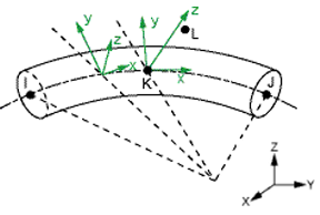
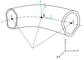
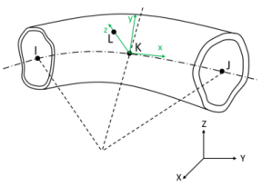
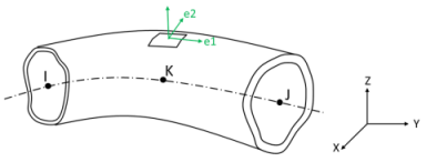
A general description of the element coordinate system is available in Coordinate Systems. Following is information about specific coordinate systems as they apply to ELBOW290 Structural Elbow.
Beam Coordinate Systems
The beam coordinate systems (x-y-z) are used for defining beam offsets and diametral temperature gradients.
 No orientation node (default) |
 Using orientation node L |
The x axis is always the axial direction pointing from node I to node J. The optional orientation node L, if used, defines a plane containing the x and z axes at node K. If this element is used in a large-deflection analysis, the location of the orientation node L is used only to initially orient the element.
When no orientation node is used, z is perpendicular to the curvature plane, uniquely determined by the I, J, and K nodes. If I, J, and K are co-linear, the y axis is automatically calculated to be parallel to the global X-Y plane. In cases where the element is parallel to the global Z axis (or within a 0.01 percent slope of the axis), the element y axis is oriented parallel to the global Y axis.
For information about orientation nodes and beam meshing, see Generating a Beam Mesh With Orientation Nodes in the Modeling and Meshing Guide. See Quadratic Elements (Midside Nodes) in the same document for information about midside nodes. For details about generating the optional orientation node L automatically, see the LMESH and LATT command descriptions.
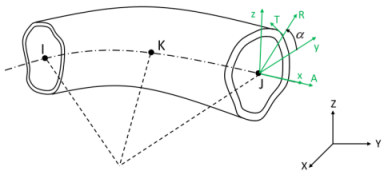
Local Cylindrical Coordinate Systems
The cylindrical coordinate systems (A-R-T) are used for defining internal section motions (that is, axial-A, radial-R, and hoop-T displacements and rotations).
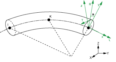
The cylindrical systems are always created from the default beam coordinate systems (beam system without orientation node L), with A being the same as beam axis x, and an angle α (0 < α < 360 degrees) from R to the beam axis y.
Element and Layer Coordinate Systems
The element coordinate systems (e1-e2-e3) are defined at the mid-surfaces of the pipe wall. The e1, e2, and e3 axes are parallel respectively to cylindrical axes A, T, and R in the undeformed configuration. Each element coordinate system is updated independently to account for large material rotation during a geometrically nonlinear analysis. Support is not available for user-defined element coordinate systems.

The layer coordinate systems (L1-L2-L3) are identical to the element coordinate system if no layer orientation angles are specified; otherwise, the layer coordinate system can be generated by rotating the corresponding element coordinate system about the shell normal (axis e3). Material properties are defined in the layer systems; therefore, the layer system is also called the material coordinate system.
ELBOW290 Structural Elbow Input Data
The geometry and node locations for ELBOW290 Structural Elbow are shown in Figure 290.1: ELBOW290 Structural Elbow Geometry. The element is defined by nodes I, J, and K in the global coordinate system.
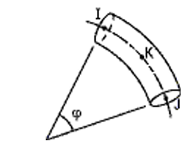
When using ELBOW290 Structural Elbow, the subtended angle
 should not exceed 45 degrees.
ELBOW290 Structural Elbow Cross Sections
The element is a one-dimensional line element in space. The cross-section details are provided separately (via the SECDATA command). A section is associated with the element by specifying the section ID number (SECNUM). A section number is an independent element attribute.
ELBOW290 Structural Elbow can only be associated with the pipe cross section (SECTYPE,,PIPE). For elements with homogeneous materials, the material of the pipe is defined as an element attribute (MAT).
The layup of a composite pipe can be defined with a shell section (SECTYPE). Shell section commands provide the input options for specifying the thickness, material, orientation and number of integration points through the thickness of the layers. The program obtains the actual layer thicknesses used for ELBOW290 Structural Elbow element calculations (by scaling the input layer thickness) so that they are consistent with the total wall thickness given by the pipe section. A single-layer shell section definition is possible, allowing flexibility with regard to the number of integration points used and other options.
For shell section input, you can designate the number of integration points (1, 3, 5, 7, or 9) located through the thickness of each layer. When only one integration point is specified, the point is always located midway between the top and bottom surfaces. If three or more points are specified, one point is located on the top surface, one point is located on the bottom surface, and the remaining points are distributed at equal distances between the top and bottom points. The default number of integration points for each layer is 3. When a single layer is defined and plasticity is present, however, the number of integration points is changed to a minimum of five during solution.
In "Element and Layer Coordinate Systems", the layer coordinate system can be obtained by rotating the corresponding element coordinate system about the shell normal (axis e3) by angle θ (in degrees). The value of θ for each layer is given by the SECDATA command input for the shell section.
For details about associating a shell section with a pipe section, see the SECDATA command documentation.
Cross-Section Deformation
The level of accuracy in elbow cross-sectional deformation is given by the
number of Fourier terms around the circumference of the cross section. The
accuracy can be adjusted via KEYOPT(2) = n, where
n is an integer value from 0 through 8, as
follows:
| KEYOPT(2) = 0 -- Only uniform radial expansion and transverse shears through the pipe wall are allowed. Suitable for simulating straight pipes without undergoing bending. |
| KEYOPT(2) = 1 -- Radial expansion and transverse shears are allowed to vary along the circumference to account for bending. Suitable for straight pipes in small-deformation analysis. |
| KEYOPT(2) = 2 through 8 -- Allow general section deformation, including radial expansion, ovalization, and warping. Suitable for curved pipes or straight pipes in large-deformation analysis. The default is KEYOPT(2) = 2. Higher values for KEYOPT(2) may be necessary for pipes with thinner walls, as they are more susceptible to complex cross-section deformation than are pipes with thicker walls. |
Element computation becomes more intensive as the value of KEYOPT(2) increases. Use a KEYOPT(2) value that offers an optimal balance between accuracy and computational cost.
Cross-Section Constraints
The constraints on the elbow cross-section can be applied at the element nodes I, J, and K with the following section degrees of freedom labels:
| SE – section radial motion (as occurs during expansion or ovalization, for example) |
| SO – section tangential motion (as occurs during ovalization, for example) |
| SW – section axial motion (as occurs during warping, for example) |
| SRA – local shell normal rotation about cylindrical axis A |
| SRT – local shell normal rotation about cylindrical axis T |
| SECT – all section deformation |

Only fixed cross-section constraints are allowed via the D
command. Delete section constraints via the DDELE command.
For example, to constrain the warping and ovalization of the cross-section at
node n, issue this command:
D, n,SW,,,,,SO
To allow only the radial expansion of the cross-section, use the following commands:
It is not practical to maintain the continuity of cross-section deformation between two adjacent elements joined at a sharp angle. For such cases, ANSYS, Inc. recommends coupling the nodal displacements and rotations but leaving the cross-section deformation uncoupled. The ELBOW command can automate the process by uncoupling the cross-section deformation for any adjacent elements with cross-sections intersecting at an angle greater than 20 degrees.
ELBOW290 Structural Elbow Transverse Shear Stiffness
ELBOW290 Structural Elbow includes the effects of transverse shear deformation through the pipe wall. The transverse shear stiffness of the element is a 2 x 2 matrix, as shown:

For a single-layer elbow with isotropic material, default transverse shear stiffnesses are as follows:

where k = 5/6, G = shear modulus, and h = pipe wall thickness.
You can override the default transverse shear stiffness values by assigning different values via the SECCONTROL command for the shell section.
ELBOW290 Structural Elbow Loads
Element loads are described in Nodal Loading. Forces are applied at the nodes. By default, ELBOW290 Structural Elbowelement nodes are located at the center of the cross-section. Use the SECOFFSET command's OFFSETY and OFFSETZ arguments for the pipe section to define locations other than the centroid for force application.
Pressure Input
Internal and external pressures are input on an average basis over the element. Lateral pressures are input as force per unit length. End "pressures" are input as forces.
To input surface-load information on the element faces, issue the SFE command
On faces 1 and 2, internal and external pressures are input, respectively, on an average basis over the element.
On face 3, the input (VAL1) is the global Z
coordinate of the free surface of the internal fluid of the pipe. Specify this
value with ACEL,0,0,ACEL_Z, where
ACEL_Z is a positive number. The free surface
coordinate is used for the internal mass and pressure effects. If
VAL1 on the SFE command is
zero, no fluid inside of the pipe is considered. If the internal fluid free
surface should be at Z = 0, use a very small number instead. The pressure
calculation presumes that the fluid density above an element to the free surface
is constant. For cases where the internal fluid consists of more than one type
of fluid (such as oil over water), the free surface coordinate of the elements
in the fluids below the top fluid need to be adjusted (lowered) to account for
the less dense fluid(s) above them.
The internal fluid mass is assumed to be lumped along the centerline of the pipe, so as the centerline of a horizontal pipe moves across the free surface, the mass changes in step-function fashion. The free surface location is stepped, even if you specify ramped loading (KBC,0).
Pressures may be input as surface loads on the element faces as shown by the circled numbers in the following illustration. Positive pressures act into the pipe wall.

The end-cap pressure effect is included by default. The end-cap effect on one or both ends of the element can be deactivated via KEYOPT(6). When subjected to internal and external pressures, ELBOW290 Structural Elbow with end caps (KEYOPT(6) = 0) is always in equilibrium; that is, no net forces are produced. Without end caps (KEYOPT(6) = 1), the element is also in equilibrium except for the case when the element is curved. With end caps only at one end (KEYOPT(6) = 2 or 3), the element is obviously not in equilibrium.
Pressure Load Stiffness
The effects of pressure load stiffness are included by default for this element. If an unsymmetric matrix is needed for pressure load stiffness effects, issue an NROPT,UNSYM command.
Temperatures
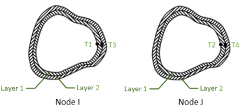
When KEYOPT(1) = 0, a layer-wise pattern is used. T1 and T2 are temperatures
at inner wall, T3 and T4 and the interface temperatures between layer 1 and
layer 2, ending with temperatures at the exterior of the pipe. All undefined
temperatures are default to TUNIF. If exactly (NL +
1) temperatures are given (where NL is the number of
layers), then one temperature is taken as the uniform temperature at the bottom
of each layer, with the last temperature for the exterior of the pipe.

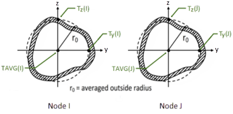
When KEYOPT(1) = 1, temperatures can be input as element body loads at three locations at both end nodes of the element so that the temperature varies linearly in the beam y axis and z axis directions. At both ends, the element temperatures are input at the section centroid (TAVG), at the outer radius from the centroid in the element y direction (Ty), and at the outer radius from the centroid in the element z direction (Tz). The first coordinate temperature TAVG defaults to TUNIF. If all temperatures after the first are unspecified, they default to the first. If all temperatures at node I are input, and all temperatures at node J are unspecified, the node J temperatures default to the corresponding node I temperatures. For any other input pattern, unspecified temperatures default to TUNIF. The following graphic illustrates temperature input when KEYOPT(1) = 1:

ELBOW290 Structural Elbow Input Summary
- Nodes
I, J, K, and L (the optional orientation node)
- Degrees of Freedom
UX, UY, UZ, ROTX, ROTY, ROTZ - Section Information
Accessed via SECTYPE,,PIPE and SECDATA commands. - Material Properties
TB command: See Element Support for Material Models for this element. MP command: EX, EY, EZ, (PRXY, PRYZ, PRXZ, or NUXY, NUYZ, NUXZ), ALPX, ALPY, ALPZ (or CTEX, CTEY, CTEZ or THSX, THSY, THSZ), DENS, GXY, GYZ, GXZ, ALPD Specify BETD and DMPR only once for the element. (Issue the MAT command to assign the material property set.) REFT may be specified once for the element, or it may be assigned on a per-layer basis. - Surface Loads
- Pressure --
face 1- Internal pressure face 2 - External pressure face 3 - Z coordinate of free surface of fluid on inside of pipe
- Body Loads
- Temperatures --
For KEYOPT(1) = 0 -- T1, T2 (at bottom of layer 1), T3, T4 (between layers 1-2); similarly for between next layers, ending with temperatures at top of layer NL(2 * (NL+ 1) maximum).For KEYOPT(1) = 1 -- TAVG(I), Ty(I), Tz(I), TAVG(J), Ty(J), Tz(J)
- Special Features
Birth and death Large deflection Large strain Nonlinear stabilization Stress stiffening - KEYOPT(1)
Temperature input:
- 0 --
Layerwise input
- 1 --
Diametral gradient
- KEYOPT(2)
Number of Fourier terms (used for cross-sectional flexibility):
- 0 --
Uniform radial expansion
- 1 --
Nonuniform radial expansion to account for bending
- 2 through 8 --
General section deformation (default = 2)
- KEYOPT(6)
End cap loads:
- 0 --
Internal and external pressures cause loads on end caps
- 1 --
Internal and external pressures do not cause loads on end caps
- 2 --
Internal and external pressures cause loads on element node I
- 3 --
Internal and external pressures cause loads on element node J
- KEYOPT(8)
Specify layer data storage:
- 0 --
For multi-layer elements, store data for bottom of bottom layer and top of top layer. For single-layer elements, store data for TOP and BOTTOM. (Default)
- 1 --
Store data for TOP and BOTTOM, for all layers (multilayer elements)
- 2 --
Store data for TOP, BOTTOM, and MID for all layers; applies to single-layer and multilayer elements. (The volume of data may be considerable.)
- KEYOPT(10)
Thickness normal stress (Sz) output option:
- 0 --
Sz not modified (default, Sz = 0)
- 1 --
Recover and output Sz from applied pressure load
ELBOW290 Structural Elbow Output Data
The solution output associated with these elements is in two forms:
Nodal displacements and reactions included in the overall nodal solution
Additional element output as described in Table 290.1: ELBOW290 Structural Elbow Output Definitions
Integration Stations
Integration stations along the length and within the cross-section of the elbow are shown in Figure 290.2: ELBOW290 Structural Elbow Element Integration Stations.

Element solution is available at all integration points through element printout (OUTPR). Solution via the POST1 postprocessor is available at element nodes and selected section integration locations (see KEYOPT(8) settings for more details).
Stress Output
Several items are illustrated in Figure 290.3: ELBOW290 Structural Elbow Stress Output:

KEYOPT(8) controls the amount of data output to the results file for processing with the LAYER command. Interlaminar shear stress is available at the layer interfaces. KEYOPT(8) must be set to either 1 or 2 to output these stresses in the POST1 postprocessor. A general description of solution output is given in Solution Output. See the Basic Analysis Guide for ways to review results.
KEYOPT(10) = 1 outputs normal stress component Sz, where z is shell normal direction. The element uses a plane-stress formulation that always leads to zero thickness normal stress. With KEYOPT(10) = 1, Sz is independently recovered during the element solution output from the applied pressure load.
The element shell stress resultants (N11, M11, Q13, etc.) are parallel to the element coordinate system (e1-e2-e3), as are the shell membrane strains and curvatures (ε11, κ11, γ13, etc.) of the element. Shell stress resultants and generalized shell strains are available via the SMISC option at the element end nodes I and J only.
ELBOW290 Structural Elbow also outputs beam-related stress resultants (Fx, My, TQ, etc) and linearized stresses (SDIR, SByT, SByB, etc) at two element end nodes I and J to SMISC records. Beam stress resultants and linearized stresses are parallel to the beam coordinate system (x-y-z).
Linearized Stress
It is customary in pipe design to employ components of axial stress that contribute to axial loads and bending in each direction separately. Therefore, ELBOW290 Structural Elbow provides a linearized stress output as part of its SMISC output record, as indicated in the following definitions:
SDIR is the stress component due to axial load.
SDIR = Fx/A, where Fx is the axial load (SMISC quantities 1 and 36) and A is the area of the cross section (SMISC quantities 7 and 42).
SByT and SByB are bending stress components.
| SByT = -Mz * ymax / Izz |
| SByB = -Mz * ymin / Izz |
| SBzT = My * zmax / Iyy |
| SBzB = My * zmin / Iyy |
where My, Mz are bending moments (SMISC quantities 2,37,3,38). Coordinates ymax, ymin, zmax, and zmin are the maximum and minimum y, z coordinates in the cross section measured from the centroid. Values Iyy and Izz are moments of inertia of the cross section.
The reported stresses are strictly valid only for elastic behavior of members. ELBOW290 Structural Elbow always employs combined stresses in order to support nonlinear material behavior. When the elements are associated with nonlinear materials, the component stresses can at best be regarded as linearized approximations and should be interpreted with caution.
ELBOW290 does not provide extensive element printout.
Because the POST1 postprocessor provides more comprehensive output processing tools,
ANSYS, Inc. suggests issuing the OUTRES command to ensure that
the required results are stored in the database. To view 3-D deformed shapes for
ELBOW290, issue an OUTRES,MISC or
OUTRES,ALL command for static or transient analyses. To view
3-D mode shapes for a modal or eigenvalue buckling analysis, expand the modes with
element results calculation active via the MXPAND command's
Elcalc = YES option.
ELBOW290 Structural Elbow Output Definitions
In the table below, the O column indicates the availability of the items in the file Jobname.OUT. The R column indicates the availability of the items in the results file.
In either the O or R columns, “Y” indicates that the item is always available, a number refers to a table footnote that describes when the item is conditionally available, and “-” indicates that the item is not available.
For the stress and strain components, X refers to axial, Y refers to hoop, and Z refers to radial.
Table 290.1: ELBOW290 Structural Elbow Output Definitions
| Name | Definition | O | R |
|---|---|---|---|
| EL | Element number | Y | Y |
| NODES | Element connectivity | - | Y |
| MAT | Material number | - | Y |
| THICK | Average wall thickness | - | Y |
| AREA | Area of cross-section | - | Y |
| XC, YC, ZC | Location where results are reported | - | 1 |
| LOCI:X, Y, Z | Integration point locations | - | 2 |
| TEMP | T1, T2 at bottom of layer 1, T3, T4 between layers 1-2, similarly
for between next layers, ending with temperatures at top of layer
NL (2 *
(NL + 1) maximum) | - | Y |
| LOC | TOP, MID, BOT, or integration point location | - | 3 |
| S:X, Y, Z, XY, YZ, XZ | Stresses | 5 | 3 |
| S:INT | Stress intensity | - | 3 |
| S:EQV | Equivalent stress | - | 3 |
| EPEL:X, Y, Z, XY | Elastic strains | 5 | 3 |
| EPEL:EQV | Equivalent elastic strains [4] | - | 3 |
| EPTH:X, Y, Z, XY | Thermal strains | 5 | 3 |
| EPTH:EQV | Equivalent thermal strains [4] | - | 3 |
| EPPL:X, Y, Z, XY | Average plastic strains | 5 | 6 |
| EPPL:EQV | Equivalent plastic strains [4] | - | 6 |
| EPCR:X, Y, Z, XY | Average creep strains | 5 | 6 |
| EPCR:EQV | Equivalent creep strains [4] | - | 6 |
| EPTO:X, Y, Z, XY | Total mechanical strains (EPEL + EPPL + EPCR) | 5 | - |
| EPTO:EQV | Total equivalent mechanical strains (EPEL + EPPL + EPCR) | - | - |
| NL:SEPL | Plastic yield stress | - | 6 |
| NL:SRAT | Plastic yielding (1 = actively yielding, 0 = not yielding) | - | 6 |
| NL:HPRES | Hydrostatic pressure | - | 6 |
| NL:EPEQ | Accumulated equivalent plastic strain | - | 6 |
| NL:CREQ | Accumulated equivalent creep strain | - | 6 |
| NL:PLWK | Plastic work/volume | - | 6 |
| SEND:ELASTIC, PLASTIC, CREEP | Strain energy densities | - | 6 |
| Fx | Section axial force | - | Y |
| My, Mz | Section bending moments | - | Y |
| TQ | Section torsional moment | - | Y |
| SFy, SFz | Section shear forces | - | Y |
| INT PRESS | Internal pressure at integration point | Y | Y |
| EXT PRESS | External pressure at integration point | Y | Y |
| EFFECTIVE TENS | Effective tension at integration point | Y | Y |
| MAX HOOP STRESS | Maximum hoop stress at integration point | Y | Y |
| SDIR | Axial direct stress | - | Y |
| SByT | Bending stress on the element +y side of the pipe | - | Y |
| SByB | Bending stress on the element -y side of the pipe | - | Y |
| SBzT | Bending stress on the element +z side of the pipe | - | Y |
| SBzB | Bending stress on the element -z side of the pipe | - | Y |
| N11, N22, N12 | Wall in-plane forces (per unit length) | - | Y |
| M11, M22, M12 | Wall out-of-plane moments (per unit length) | - | Y |
| Q13, Q23 | Wall transverse shear forces (per unit length) | - | Y |
| ε11, ε22, ε12 | Wall membrane strains | - | Y |
| κ11, κ22, κ12 | Wall curvatures | - | Y |
| γ13, γ23 | Wall transverse shear strains | - | Y |
SVAR:1, 2, ... , N
| State variables | - | 7 |
| OVAL | Ovalization (Dmax - Dmin) / D (where D = diameter) | - | Y |
Available only at the centroid as a *GET item.
Available via an OUTRES,LOCI command only.
The subsequent stress solution repeats for top, middle, and bottom surfaces.
The equivalent strains use an effective Poisson's ratio. For elastic and thermal, you set the value (MP,PRXY). For plastic and creep, the program sets the value at 0.5.
Stresses, total strains, plastic strains, elastic strains, creep strains, and thermal strains in the element coordinate system are available for output (at all section points through thickness). If layers are in use, the results are in the layer coordinate system.
Nonlinear solution output for top, middle, and bottom surfaces, if the element has a nonlinear material, or if large-deflection effects are enabled (NLGEOM,ON) for SEND.
Available only if the
UserMatsubroutine and TB,STATE command are used.
More output is described via the PRESOL and *GET,,SECR commands in POST1.
ELBOW290 Structural Elbow Item and Sequence Numbers
Table 290.2: ELBOW290 Structural Elbow Item and Sequence Numbers lists output available for the ETABLE and ESOL commands using the Sequence Number method. See Creating an Element Table in the Basic Analysis Guide and The Item and Sequence Number Table in this reference for more information. The table uses the following notation:
- Name
output quantity as defined in Table 290.1: ELBOW290 Structural Elbow Output Definitions
- Item
predetermined Item label for ETABLE
- I,J
sequence number for data at nodes I and J
Table 290.2: ELBOW290 Structural Elbow Item and Sequence Numbers
| Output Quantity Name | ETABLE and ESOL Command Input | ||
|---|---|---|---|
| Item | I | J | |
| Fx | SMISC | 1 | 36 |
| My | SMISC | 2 | 37 |
| Mz | SMISC | 3 | 38 |
| TQ | SMISC | 4 | 39 |
| SFz | SMISC | 5 | 40 |
| SFy | SMISC | 6 | 41 |
| SDIR | SMISC | 8 | 43 |
| SByT | SMISC | 9 | 44 |
| SByB | SMISC | 10 | 45 |
| SBzT | SMISC | 11 | 46 |
| SBzB | SMISC | 12 | 47 |
| N11 | SMISC | 14 | 49 |
| N22 | SMISC | 15 | 50 |
| N12 | SMISC | 16 | 51 |
| M11 | SMISC | 17 | 52 |
| M22 | SMISC | 18 | 53 |
| M12 | SMISC | 19 | 54 |
| Q13 | SMISC | 20 | 55 |
| Q23 | SMISC | 21 | 56 |
| ε11 | SMISC | 22 | 57 |
| ε22 | SMISC | 23 | 58 |
| ε12 | SMISC | 24 | 59 |
| κ11 | SMISC | 25 | 60 |
| κ22 | SMISC | 26 | 61 |
| κ12 | SMISC | 27 | 62 |
| γ13 | SMISC | 28 | 63 |
| γ23 | SMISC | 29 | 64 |
| INT PRESS | SMISC | 71 | 75 |
| EXT PRESS | SMISC | 72 | 76 |
| EFFECTIVE TENS | SMISC | 73 | 77 |
| MAX HOOP STRESS | SMISC | 74 | 78 |
| AREA | NMISC | 1 | 6 |
| THICK | NMISC | 2 | 7 |
| OVAL | NMISC | 3 | 8 |
ELBOW290 Structural Elbow Assumptions and Restrictions
The element cannot have zero length.
Cross-sections must be round initially.
Wall thickness and outside diameter must be uniform within the element.
Zero wall thickness is not allowed. (Zero thickness layers are allowed.)
In a nonlinear analysis, the solution is terminated if the thickness at any integration point vanishes (within a small numerical tolerance).
This element works best with the full Newton-Raphson solution scheme (the default behavior in solution control).
No slippage is assumed between the element layers. Shear deflections are included in the element; however, normals to the center wall surface before deformation are assumed to remain straight after deformation.
If multiple load steps are used, the number of layers must remain unchanged between load steps.
If the layer material is hyperelastic, the layer orientation angle has no effect.
Stress stiffening is always included in geometrically nonlinear analyses (NLGEOM,ON). Apply prestress effects via a PSTRES command.
The through-thickness stress SZ is always zero.
The effects of fluid motion inside the pipe are ignored.
ELBOW290 Generalized Tube Description
The ELBOW290 Generalized Tube is suitable for modeling thin to moderately thick-walled tubular structures with arbitrary cross sections. The wall can be either homogenous or a layered composite. The cross-sectional geometry, including the wall thickness, can vary along the element length. Wall thickness must be uniform within the cross section, however.
A general description of the element coordinate system is available in Coordinate Systems. Following is information about specific coordinate systems as they apply to ELBOW290 Generalized Tube .
Beam Coordinate Systems
The beam coordinate systems (x-y-z) are used for orienting the generalized tube section. The beam coordinate systems are used also for defining beam offsets (see SECOFFSET command) and diametral temperature gradients.
 No orientation node (default) |
 Using orientation node L |
The x axis is always the axial direction pointing from node I to node J. The optional orientation node L, if used, defines a plane containing the x and z axes at node K. If this element is used in a large-deflection analysis, the location of the orientation node L is used only to initially orient the element.
When no orientation node is used, z is perpendicular to the curvature plane, uniquely determined by the I, J, and K nodes. If I, J, and K are co-linear, the y axis is automatically calculated to be parallel to the global X-Y plane. In cases where the element is parallel to the global Z axis (or within a 0.01 percent slope of the axis), the element y axis is oriented parallel to the global Y axis.
For information about orientation nodes and beam meshing, see Generating a Beam Mesh With Orientation Nodes in the Modeling and Meshing Guide. See Quadratic Elements (Midside Nodes) in the same document for information about midside nodes. For details about generating the optional orientation node L automatically, see the LMESH and LATT command descriptions.
Local Cylindrical Coordinate Systems
The cylindrical coordinate systems (A-R-T) are used for defining internal section motions (that is, axial-A, radial-R, and hoop-T displacements and rotations).
The cylindrical systems are always created from the default beam coordinate systems (beam system without orientation node L), with A being the same as beam axis x, and an angle α (0 < α < 360 degrees) from R to the beam axis y.
Element and Layer Coordinate Systems
The element coordinate systems (e1-e2-e3) are defined at the mid-surfaces of the pipe wall. The e1, e2, and e3 axes are parallel respectively to cylindrical axes A, T, and R in the undeformed configuration. Each element coordinate system is updated independently to account for large material rotation during a geometrically nonlinear analysis. Support is not available for user-defined element coordinate systems.
The layer coordinate systems (L1-L2-L3) are identical to the element coordinate system if no layer orientation angles are specified; otherwise, the layer coordinate system can be generated by rotating the corresponding element coordinate system about the shell normal (axis e3). Material properties are defined in the layer systems; therefore, the layer system is also called the material coordinate system.
ELBOW290 Generalized Tube Input Data
The geometry and node locations for ELBOW290 Generalized Tube are shown in Figure 290.1: ELBOW290 Structural Elbow Geometry. The element is defined by nodes I, J, and K in the global coordinate system.
When using ELBOW290 Generalized Tube, the subtended angle
 should not exceed 45 degrees.
ELBOW290 Generalized Tube Cross Sections
The element is a one-dimensional line element in space. The cross-section details are provided separately (via the SECDATA command). A section is associated with the element by specifying the section ID number (SECNUM). A section number is an independent element attribute.
ELBOW290 Generalized Tube can be associated with the pipe cross section (SECTYPE,,PIPE) or tapered pipe cross section (SECTYPE,,TAPER). For details about creating generalized tube sections, see Defining a Tapered Beam or Pipe and Defining a Noncircular Pipe in the Structural Analysis Guide.
The layup of a composite pipe can be defined with a shell section (SECTYPE). Shell section commands provide the input options for specifying the thickness, material, orientation and number of integration points through the thickness of the layers. The program obtains the actual layer thicknesses used for ELBOW290 Generalized Tube element calculations (by scaling the input layer thickness) so that they are consistent with the total wall thickness given by the pipe section. A single-layer shell section definition is possible, allowing flexibility with regard to the number of integration points used and other options.
For shell section input, you can designate the number of integration points (1, 3, 5, 7, or 9) located through the thickness of each layer. When only one integration point is specified, the point is always located midway between the top and bottom surfaces. If three or more points are specified, one point is located on the top surface, one point is located on the bottom surface, and the remaining points are distributed at equal distances between the top and bottom points. The default number of integration points for each layer is 3. When a single layer is defined and plasticity is present, however, the number of integration points is changed to a minimum of five during solution.
In "Element and Layer Coordinate Systems", the layer coordinate system can be obtained by rotating the corresponding element coordinate system about the shell normal (axis e3) by angle θ (in degrees). The value of θ for each layer is given by the SECDATA command input for the shell section.
For details about associating a shell section with a pipe section, see the SECDATA command documentation.
For elements with homogeneous materials, the material of the pipe is defined as an element attribute (MAT).
Cross-Section Deformation
The level of accuracy in elbow cross-sectional deformation is given by the
number of Fourier terms around the circumference of the cross section. The
accuracy can be adjusted via KEYOPT(2) = n, where
n is an integer value from 0 through 8, as
follows:
| KEYOPT(2) = 0 -- Only uniform radial expansion and transverse shears through the pipe wall are allowed. Suitable for simulating straight pipes without undergoing bending. |
| KEYOPT(2) = 1 -- Radial expansion and transverse shears are allowed to vary along the circumference to account for bending. Suitable for straight pipes in small-deformation analysis. |
| KEYOPT(2) = 2 through 8 -- Allow general section deformation, including radial expansion, ovalization, and warping. Suitable for curved pipes or straight pipes in large-deformation analysis. The default is KEYOPT(2) = 2. Higher values for KEYOPT(2) may be necessary for pipes with thinner walls, as they are more susceptible to complex cross-section deformation than are pipes with thicker walls. |
Element computation becomes more intensive as the value of KEYOPT(2) increases. Use a KEYOPT(2) value that offers an optimal balance between accuracy and computational cost.
Cross-Section Constraints
The constraints on the elbow cross-section can be applied at the element nodes I, J, and K with the following section degrees of freedom labels:
| SE – section radial motion (as occurs during expansion or ovalization, for example) |
| SO – section tangential motion (as occurs during ovalization, for example) |
| SW – section axial motion (as occurs during warping, for example) |
| SRA – local shell normal rotation about cylindrical axis A |
| SRT – local shell normal rotation about cylindrical axis T |
| SECT – all section deformation |
Only fixed cross-section constraints are allowed via the D
command. Delete section constraints via the DDELE command.
For example, to constrain the warping and ovalization of the cross-section at
node n, issue this command:
D, n,SW,,,,,SO
To allow only the radial expansion of the cross-section, use the following commands:
It is not practical to maintain the continuity of cross-section deformation between two adjacent elements joined at a sharp angle. For such cases, ANSYS, Inc. recommends coupling the nodal displacements and rotations but leaving the cross-section deformation uncoupled. The ELBOW command can automate the process by uncoupling the cross-section deformation for any adjacent elements with cross-sections intersecting at an angle greater than 20 degrees.
ELBOW290 Generalized Tube Transverse Shear Stiffness
ELBOW290 Generalized Tube includes the effects of transverse shear deformation through the pipe wall. The transverse shear stiffness of the element is a 2 x 2 matrix, as shown:

For a single-layer elbow with isotropic material, default transverse shear stiffnesses are as follows:

where k = 5/6, G = shear modulus, and h = pipe wall thickness.
You can override the default transverse shear stiffness values by assigning different values via the SECCONTROL command for the shell section.
ELBOW290 Generalized Tube Loads
Element loads are described in Nodal Loading. Forces are applied at the nodes. By default, ELBOW290 Generalized Tube element nodes are located at the center of the cross-section. Use the SECOFFSET command's OFFSETY and OFFSETZ arguments for the pipe section to define locations other than the centroid for force application.
Pressure Input
Internal and external pressures are input on an average basis over the element. Lateral pressures are input as force per unit length. End "pressures" are input as forces.
To input surface-load information on the element faces, issue the SFE command
On faces 1 and 2, internal and external pressures are input, respectively, on an average basis over the element.
On face 3, the input (VAL1) is the global Z
coordinate of the free surface of the internal fluid of the pipe. Specify this
value with ACEL,0,0,ACEL_Z, where
ACEL_Z is a positive number. The free surface
coordinate is used for the internal mass and pressure effects. If
VAL1 on the SFE command is
zero, no fluid inside of the pipe is considered. If the internal fluid free
surface should be at Z = 0, use a very small number instead. The pressure
calculation presumes that the fluid density above an element to the free surface
is constant. For cases where the internal fluid consists of more than one type
of fluid (such as oil over water), the free surface coordinate of the elements
in the fluids below the top fluid need to be adjusted (lowered) to account for
the less dense fluid(s) above them.
The internal fluid mass is assumed to be lumped along the centerline of the pipe, so as the centerline of a horizontal pipe moves across the free surface, the mass changes in step-function fashion. The free surface location is stepped, even if you specify ramped loading (KBC,0).
Pressures may be input as surface loads on the element faces as shown by the circled numbers in the following illustration. Positive pressures act into the pipe wall.
The end-cap pressure effect is included by default. The end-cap effect on one or both ends of the element can be deactivated via KEYOPT(6). When subjected to internal and external pressures, ELBOW290 Generalized Tube with end caps (KEYOPT(6) = 0) is always in equilibrium; that is, no net forces are produced. Without end caps (KEYOPT(6) = 1), the element is also in equilibrium except for the case when the element is curved. With end caps only at one end (KEYOPT(6) = 2 or 3), the element is obviously not in equilibrium.
Pressure Load Stiffness
The effects of pressure load stiffness are included by default for this element. If an unsymmetric matrix is needed for pressure load stiffness effects, issue an NROPT,UNSYM command.
Temperatures
When KEYOPT(1) = 0, a layer-wise pattern is used. T1 and T2 are temperatures
at inner wall, T3 and T4 and the interface temperatures between layer 1 and
layer 2, ending with temperatures at the exterior of the pipe. All undefined
temperatures are default to TUNIF. If exactly (NL +
1) temperatures are given (where NL is the number of
layers), then one temperature is taken as the uniform temperature at the bottom
of each layer, with the last temperature for the exterior of the pipe.
When KEYOPT(1) = 1, temperatures can be input as element body loads at three locations at both end nodes of the element so that the temperature varies linearly in the beam y axis and z axis directions. At both ends, the element temperatures are input at the section centroid (TAVG), at the outer radius from the centroid in the element y direction (Ty), and at the outer radius from the centroid in the element z direction (Tz). The first coordinate temperature TAVG defaults to TUNIF. If all temperatures after the first are unspecified, they default to the first. If all temperatures at node I are input, and all temperatures at node J are unspecified, the node J temperatures default to the corresponding node I temperatures. For any other input pattern, unspecified temperatures default to TUNIF. The following graphic illustrates temperature input when KEYOPT(1) = 1:
ELBOW290 Generalized Tube Input Summary
- Nodes
I, J, K, and L (the optional orientation node)
- Degrees of Freedom
UX, UY, UZ, ROTX, ROTY, ROTZ - Section Information
Accessed via SECTYPE,,PIPE or SECTYPE,,TAPER, and SECDATA commands. - Material Properties
TB command: See Element Support for Material Models for this element. MP command: EX, EY, EZ, (PRXY, PRYZ, PRXZ, or NUXY, NUYZ, NUXZ), ALPX, ALPY, ALPZ (or CTEX, CTEY, CTEZ or THSX, THSY, THSZ), DENS, GXY, GYZ, GXZ, ALPD Specify BETD only once for the element. (Issue the MAT command to assign the material property set.) REFT may be specified once for the element, or it may be assigned on a per-layer basis. - Surface Loads
- Pressure --
face 1- Internal pressure face 2 - External pressure face 3 - Z coordinate of free surface of fluid on inside of pipe
- Body Loads
- Temperatures --
For KEYOPT(1) = 0 -- T1, T2 (at bottom of layer 1), T3, T4 (between layers 1-2); similarly for between next layers, ending with temperatures at top of layer NL(2 * (NL+ 1) maximum).For KEYOPT(1) = 1 -- TAVG(I), Ty(I), Tz(I), TAVG(J), Ty(J), Tz(J)
- Special Features
Birth and death Large deflection Large strain Nonlinear stabilization Stress stiffening - KEYOPT(1)
Temperature input:
- 0 --
Layerwise input
- 1 --
Diametral gradient
- KEYOPT(2)
Number of Fourier terms (used for cross-sectional flexibility)
- 0 --
Uniform radial expansion
- 1 --
Nonuniform radial expansion to account for bending
- 2 through 8 --
General section deformation (default = 2)
- KEYOPT(6)
End cap loads:
- 0 --
Internal and external pressures cause loads on end caps
- 1 --
Internal and external pressures do not cause loads on end caps
- 2 --
Internal and external pressures cause loads on element node I
- 3 --
Internal and external pressures cause loads on element node J
- KEYOPT(8)
Specify layer data storage:
- 0 --
Store data for bottom of bottom layer and top of top layer (multilayer elements) (default)
- 1 --
Store data for TOP and BOTTOM, for all layers (multilayer elements)
- 2 --
Store data for TOP, BOTTOM, and MID for all layers; applies to single-layer and multilayer elements. (The volume of data may be considerable.)
- KEYOPT(10)
Thickness normal stress (Sz) output option:
- 0 --
Sz not modified (default Sz = 0)
- 1 --
Recover and output Sz from applied pressure load
ELBOW290 Generalized Tube Output Data
The solution output associated with these elements is in two forms:
Nodal displacements and reactions included in the overall nodal solution
Additional element output as described in Table 290.3: ELBOW290 Generalized Tube Output Definitions.
Integration Stations
Integration stations along the length and within the cross-section of the elbow are shown in Figure 290.5: ELBOW290 Generalized Tube Element Integration Stations.
Element solution is available at all integration points through element printout (OUTPR). Solution via the POST1 postprocessor is available at element nodes and selected section integration locations (see KEYOPT(8) settings for more details).
Stress Output
Several items are illustrated in Figure 290.6: ELBOW290 Generalized Tube Stress Output:
KEYOPT(8) controls the amount of data output to the results file for processing with the LAYER command. Interlaminar shear stress is available at the layer interfaces. KEYOPT(8) must be set to either 1 or 2 to output these stresses in the POST1 postprocessor. A general description of solution output is given in Solution Output. See the Basic Analysis Guide for ways to review results.
KEYOPT(10) = 1 outputs normal stress component Sz, where z is shell normal direction. The element uses a plane-stress formulation that always leads to zero thickness normal stress. With KEYOPT(10) = 1, Sz is independently recovered during the element solution output from the applied pressure load.
The element shell stress resultants (N11, M11, Q13, etc.) are parallel to the element coordinate system (e1-e2-e3), as are the shell membrane strains and curvatures (ε11, κ11, γ13, etc.) of the element. Shell stress resultants and generalized shell strains are available via the SMISC option at the element end nodes I and J only.
ELBOW290 Generalized Tube also outputs beam-related stress resultants (Fx, My, TQ, etc) and linearized stresses (SDIR, SByT, SByB, etc) at two element end nodes I and J to SMISC records. Beam stress resultants and linearized stresses are parallel to the beam coordinate system (x-y-z).
Linearized Stress
It is customary in pipe design to employ components of axial stress that contribute to axial loads and bending in each direction separately. Therefore, ELBOW290 Generalized Tube provides a linearized stress output as part of its SMISC output record, as indicated in the following definitions:
SDIR is the stress component due to axial load.
SDIR = Fx/A, where Fx is the axial load (SMISC quantities 1 and 36) and A is the area of the cross section (SMISC quantities 7 and 42).
SByT and SByB are bending stress components.
| SByT = -Mz * ymax / Izz |
| SByB = -Mz * ymin / Izz |
| SBzT = My * zmax / Iyy |
| SBzB = My * zmin / Iyy |
where My, Mz are bending moments (SMISC quantities 2,37,3,38). Coordinates ymax, ymin, zmax, and zmin are the maximum and minimum y, z coordinates in the cross section measured from the centroid. Values Iyy and Izz are moments of inertia of the cross section.
The reported stresses are strictly valid only for elastic behavior of members. ELBOW290 Generalized Tube always employs combined stresses in order to support nonlinear material behavior. When the elements are associated with nonlinear materials, the component stresses can at best be regarded as linearized approximations and should be interpreted with caution.
ELBOW290 Generalized Tube does not provide extensive
element printout. Because the POST1 postprocessor provides more comprehensive output
processing tools, ANSYS, Inc. suggests issuing the OUTRES command
to ensure that the required results are stored in the database. To view 3-D deformed
shapes for ELBOW290 Generalized Tube, issue an
OUTRES,MISC or OUTRES,ALL command for
static or transient analyses. To view 3-D mode shapes for a modal or eigenvalue
buckling analysis, expand the modes with element results calculation active via the
MXPAND command's Elcalc = YES
option.
ELBOW290 Generalized Tube Output Definitions
The Element Output Definitions table uses the following notation:
The O column indicates the availability of the items in the file Jobname.OUT. The R column indicates the availability of the items in the results file.
In either the O or R columns, “Y” indicates that the item is always available, a number refers to a table footnote that describes when the item is conditionally available, and “-” indicates that the item is not available.
Table 290.3: ELBOW290 Generalized Tube Output Definitions
| Name | Definition | O | R |
|---|---|---|---|
| EL | Element number | Y | Y |
| NODES | Element connectivity | - | Y |
| MAT | Material number | - | Y |
| THICK | Average wall thickness | - | Y |
| AREA | Area of cross-section | - | Y |
| XC, YC, ZC | Location where results are reported | - | 1 |
| LOCI:X, Y, Z | Integration point locations | - | 2 |
| TEMP | T1, T2 at bottom of layer 1, T3, T4 between layers 1-2, similarly
for between next layers, ending with temperatures at top of layer
NL (2 *
(NL + 1) maximum) | - | Y |
| LOC | TOP, MID, BOT, or integration point location | - | 3 |
| S:X, Y, Z, XY, YZ, XZ | Stresses | 5 | 3 |
| S:INT | Stress intensity | - | 3 |
| S:EQV | Equivalent stress | - | 3 |
| EPEL:X, Y, Z, XY | Elastic strains | 5 | 3 |
| EPEL:EQV | Equivalent elastic strains [4] | - | 3 |
| EPTH:X, Y, Z, XY | Thermal strains | 5 | 3 |
| EPTH:EQV | Equivalent thermal strains [4] | - | 3 |
| EPPL:X, Y, Z, XY | Average plastic strains | 5 | 6 |
| EPPL:EQV | Equivalent plastic strains [4] | - | 6 |
| EPCR:X, Y, Z, XY | Average creep strains | 5 | 6 |
| EPCR:EQV | Equivalent creep strains [4] | - | 6 |
| EPTO:X, Y, Z, XY | Total mechanical strains (EPEL + EPPL + EPCR) | 5 | - |
| EPTO:EQV | Total equivalent mechanical strains (EPEL + EPPL + EPCR) | - | - |
| NL:EPEQ | Accumulated equivalent plastic strain | - | 6 |
| NL:CREQ | Accumulated equivalent creep strain | - | 6 |
| NL:SRAT | Plastic yielding (1 = actively yielding, 0 = not yielding) | - | 6 |
| NL:PLWK | Plastic work/volume | - | 6 |
| NL:HPRES | Hydrostatic pressure | - | 6 |
| SEND:ELASTIC, PLASTIC, CREEP | Strain energy densities | - | 6 |
| Fx | Section axial force | - | Y |
| My, Mz | Section bending moments | - | Y |
| TQ | Section torsional moment | - | Y |
| SFy, SFz | Section shear forces | - | Y |
| INT PRESS | Internal pressure at integration point | Y | Y |
| EXT PRESS | External pressure at integration point | Y | Y |
| EFFECTIVE TENS | Effective tension on pipe | Y | Y |
| MAX HOOP STRESS | Maximum hoop stress at integration point | Y | Y |
| SDIR | Axial direct stress | - | Y |
| SByT | Bending stress on the element +y side of the pipe | - | Y |
| SByB | Bending stress on the element -y side of the pipe | - | Y |
| SBzT | Bending stress on the element +z side of the pipe | - | Y |
| SBzB | Bending stress on the element -z side of the pipe | - | Y |
| N11, N22, N12 | Wall in-plane forces (per unit length) | - | Y |
| M11, M22, M12 | Wall out-of-plane moments (per unit length) | - | Y |
| Q13, Q23 | Wall transverse shear forces (per unit length) | - | Y |
| ε11, ε22, ε12 | Wall membrane strains | - | Y |
| κ11, κ22, κ12 | Wall curvatures | - | Y |
| γ13, γ23 | Wall transverse shear strains | - | Y |
SVAR:1, 2, ... , N
| State variables | - | 7 |
Available only at the centroid as a *GET item.
Available via an OUTRES,LOCI command only.
The subsequent stress solution repeats for top, middle, and bottom surfaces.
The equivalent strains use an effective Poisson's ratio. For elastic and thermal, you set the value (MP,PRXY). For plastic and creep, the program sets the value at 0.5.
Stresses, total strains, plastic strains, elastic strains, creep strains, and thermal strains in the element coordinate system are available for output (at all section points through thickness). If layers are in use, the results are in the layer coordinate system.
Nonlinear solution output for top, middle, and bottom surfaces, if the element has a nonlinear material, or if large-deflection effects are enabled (NLGEOM,ON) for SEND.
Available only if the
UserMatsubroutine and TB,STATE command are used.
More output is described via the PRESOL and *GET,,SECR commands in POST1.
ELBOW290 Generalized Tube Item and Sequence Numbers
Table 290.4: ELBOW290 Generalized Tube Item and Sequence Numbers lists output available for the ETABLE command using the Sequence Number method. See Creating an Element Table in the Basic Analysis Guide and The Item and Sequence Number Table in this document for more information. The output tables use the following notation:
- Name
output quantity as defined in Table 290.3: ELBOW290 Generalized Tube Output Definitions
- Item
predetermined Item label for ETABLE
- I,J
sequence number for data at nodes I and J
Table 290.4: ELBOW290 Generalized Tube Item and Sequence Numbers
| Output Quantity Name | ETABLE and ESOL Command Input | ||
|---|---|---|---|
| Item | I | J | |
| Fx | SMISC | 1 | 36 |
| My | SMISC | 2 | 37 |
| Mz | SMISC | 3 | 38 |
| TQ | SMISC | 4 | 39 |
| SFz | SMISC | 5 | 40 |
| SFy | SMISC | 6 | 41 |
| SDIR | SMISC | 8 | 43 |
| SByT | SMISC | 9 | 44 |
| SByB | SMISC | 10 | 45 |
| SBzT | SMISC | 11 | 46 |
| SBzB | SMISC | 12 | 47 |
| N11 | SMISC | 14 | 49 |
| N22 | SMISC | 15 | 50 |
| N12 | SMISC | 16 | 51 |
| M11 | SMISC | 17 | 52 |
| M22 | SMISC | 18 | 53 |
| M12 | SMISC | 19 | 54 |
| Q13 | SMISC | 20 | 55 |
| Q23 | SMISC | 21 | 56 |
| ε11 | SMISC | 22 | 57 |
| ε22 | SMISC | 23 | 58 |
| ε12 | SMISC | 24 | 59 |
| κ11 | SMISC | 25 | 60 |
| κ22 | SMISC | 26 | 61 |
| κ12 | SMISC | 27 | 62 |
| γ13 | SMISC | 28 | 63 |
| γ23 | SMISC | 29 | 64 |
| INT PRESS | SMISC | 71 | 75 |
| EXT PRESS | SMISC | 72 | 76 |
| EFFECTIVE TENS | SMISC | 73 | 77 |
| MAX HOOP STRESS | SMISC | 74 | 78 |
| AREA | NMISC | 1 | 6 |
| THICK | NMISC | 2 | 7 |
ELBOW290 Generalized Tube Assumptions and Restrictions
The element cannot have zero length.
Wall thickness must be uniform within the cross section.
Zero wall thickness is not allowed. (Zero thickness layers are allowed.)
In a nonlinear analysis, the solution is terminated if the thickness at any integration point vanishes (within a small numerical tolerance).
This element works best with the full Newton-Raphson solution scheme (the default behavior in solution control).
No slippage is assumed between the element layers. Shear deflections are included in the element; however, normals to the center wall surface before deformation are assumed to remain straight after deformation.
If multiple load steps are used, the number of layers must remain unchanged between load steps.
If the layer material is hyperelastic, the layer orientation angle has no effect.
Stress stiffening is always included in geometrically nonlinear analyses (NLGEOM,ON). Apply prestress effects via a PSTRES command.
The through-thickness stress SZ is always zero.
The effects of fluid motion inside the pipe are ignored.
ELBOW290 Product Restrictions
When used in the product(s) listed below, the stated product-specific restrictions apply to this element in addition to the general assumptions and restrictions given in the previous section.
ANSYS Mechanical Pro
Birth and death is not available.
ANSYS Mechanical Premium
Birth and death is not available.