Fracture or delamination along an interface between phases plays a major role in limiting the toughness and the ductility of the multi-phase materials, such as matrix-matrix composites and laminated composite structure. This has motivated considerable research on the failure of the interfaces. Interface delamination can be modeled by traditional fracture mechanics methods such as the nodal release technique. Alternatively, you can use techniques that directly introduce fracture mechanism by adopting softening relationships between tractions and the separations, which in turn introduce a critical fracture energy that is also the energy required to break apart the interface surfaces. This technique is called the cohesive zone material (CZM) model . The interface surfaces of the materials can be represented by a special set of interface elements or contact elements, and a CZM model can be used to characterize the constitutive behavior of the interface.
The CZM model consists of a constitutive relation between the traction T acting on the interface and the corresponding interfacial separation δ (displacement jump across the interface). The definitions of traction and separation depend on the element and the material model.
The following related topics are available:
For interface elements, the interfacial separation is defined as the displacement jump, δ (that is, the difference of the displacements of the adjacent interface surfaces):
 | (4–337) |
The definition of the separation is based on local element coordinate system, Figure 4.32: Schematic of Interface Elements. The normal of the interface is denoted as local direction n, and the local tangent direction is denoted as t. Thus:
 | (4–338) |
 | (4–339) |

The following related topics are available:
An exponential form of the CZM model (input via TB,CZM with TBOPT = EXPO), originally proposed
by Xu and Needleman([364]), uses a surface potential:
 | (4–340) |
where:
| ϕ(δ) = surface potential |
| e = 2.7182818 |
| σmax = maximum normal traction at the interface (input on TBDATA command as C1 using TB,CZM) |

|

|

|

|
The traction is defined as:
 | (4–341) |
or
 | (4–342) |
and
 | (4–343) |
From equations Equation 4–342 and Equation 4–343, we obtain the normal traction of the interface
 | (4–344) |
and the shear traction
 | (4–345) |
The normal work of separation is:
 | (4–346) |
and shear work of separation is assumed to be the same as the normal work of separation, ϕn, and is defined as:
 | (4–347) |
For the 3-D stress state, the shear or tangential separations and the tractions have two components, δt1 and δt2 in the element's tangential plane, and we have:
 | (4–348) |
The traction is then defined as:
 | (4–349) |
and
 | (4–350) |
(In POST1 and POST26 the traction, T, is output as SS and the separation, δ, is output as SD.)
The tangential direction t1 is defined along ij edge of element and the direction t2 is defined along direction perpendicular to the plane formed by n and t1. Directions t1, t2, and n follow the righthand side rule.
The bilinear CZM model (input via TB,CZM
with TBOPT = BILI) can be used with interface
elements. The model is based on the model proposed by Alfano and Crisfield [366].
Mode I Dominated Bilinear CZM Model
The Mode I dominated bilinear CZM model assumes that the separation of the material interfaces is dominated by the displacement jump normal to the interface, as shown in the following figure:
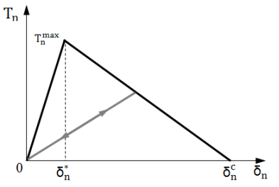
The relation between normal cohesive traction Tn and normal displacement jump δn can be expressed as:
 | (4–351) |
Where:


For Mode I dominated cohesive law, the tangential cohesive traction and tangential displacement jump behavior is assumed to follow the normal cohesive traction and normal displacement jump behavior and is expressed as:
 | (4–352) |
Were:

Mode II Dominated Bilinear CZM Model
The Mode II dominated bilinear CZM model assumes that the separation of the material interfaces is dominated by the displacement jump that is tangent to the interface, as shown in the following figure:
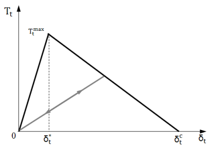
The relation between tangential cohesive traction Tt and tangential displacement jump δt can be expressed as:
 | (4–353) |
Where:


For Mode II dominated cohesive law, the normal cohesive traction and normal displacement jump behavior is assumed to follow the tangential cohesive traction and tangential displacement jump behavior and is expressed as:
 | (4–354) |
Where:

Mixed-Mode Bilinear Cohesive Zone Material Model
For bilinear cohesive law under the mixed-mode fracture, the separation of material interfaces depends on both the normal and tangential components of displacement jumps. To take into account the difference in their contributions to the separation of material interfaces, a non-dimensional effective displacement jump λ for mixed-mode fracture is defined as
 | (4–355) |
where the non-dimensional parameter β (input via the TBDATA command as C6 using TB,CZM) assigns different weights to the tangential and
normal displacement jumps.
The normal and tangential components of the cohesive tractions are expressed as:
 | (4–356) |
The damage parameter Dm associated with mixed mode bilinear cohesive law is defined as:

Where:

Fracture Mode Identification of a CZM Model
Determining the fracture mode of a CZM model is based on the input data, as follows:
| Case | Input on the TBDATA command as follows: |
| Mode I Dominated |
C1, C2, C3, C4, C5 (where C3 = -τmax) |
| Mode II/III Dominated |
C1, C2, C3, C4, C5 (where C1 = -σmax) |
| Mixed-Mode |
C1, C2, C3, C4, C5, C6 (where C1 = σmax and C3 = τmax) |
To avoid convergence difficulties, a small fictitious viscosity is introduced in cohesive zone material (CZM) models ([417]). The traction definitions are modified by adding viscous damping, as follows:
 | (4–357) |
where:
Tn = normal traction before viscous regularization
Tt = tangential traction before viscous regularization
ζ = damping coefficient (input on the TBDATA command as C1 (after defining the CZM model with the viscous regularization option [TB,CZM,,,,VREG])
Delamination with contact elements is referred to as debonding. The interfacial separation is defined in terms of contact gap or penetration and tangential slip distance. The computation of contact and tangential slip is based on the type of contact element and the location of contact detection point. The cohesive zone model can only be used for bonded contact (KEYOPT(12) = 2, 3, 4, 5, or 6) with the augmented Lagrangian method (KEYOPT(2) = 0) or the pure penalty method (KEYOPT(2) = 1). See CONTA174 - 3-D 8-Node Surface-to-Surface Contact for details.
Cohesive zone modeling with contact elements includes two different
traction separation law forms: a bilinear traction separation law
and an exponential traction separation law. Different variations of
the bilinear material models are available, with each variation being
activated by a different TBOPT value on
the TB,CZM command, as described in the following
sections:
The bilinear cohesive zone material model (input using TB,CZM with TBOPT = CBDD or
CBDE) is based on the model proposed by Alfano and Crisfield [366].
Mode I Debonding
Mode I debonding defines a mode of separation of the interface surfaces where the separation normal to the interface dominates the slip tangent to the interface. The normal contact stress (tension) and contact gap behavior is plotted in Figure 4.35: Normal Contact Stress and Contact Gap Curve for Bilinear Cohesive Zone Material. It shows linear elastic loading (OA) followed by linear softening (AC). The maximum normal contact stress is achieved at point A. Debonding begins at point A and is completed at point C when the normal contact stress reaches zero value; any further separation occurs without any normal contact stress. The area under the curve OAC is the energy released due to debonding and is called the critical fracture energy. The slope of the line OA determines the contact gap at the maximum normal contact stress and, hence, characterizes how the normal contact stress decreases with the contact gap, i.e., whether the fracture is brittle or ductile. After debonding has been initiated it is assumed to be cumulative and any unloading and subsequent reloading occurs in a linear elastic manner along line OB at a more gradual slope.

The equation for curve OAC can be written as:
 | (4–358) |
where:
| P = normal contact stress (tension) |
| Kn = normal contact stiffness |
| un = contact gap |
 = contact gap at the maximum normal
contact stress (tension) = contact gap at the maximum normal
contact stress (tension) |
 = contact gap at the completion
of debonding (input on TBDATA command as C2 using TB,CZM) = contact gap at the completion
of debonding (input on TBDATA command as C2 using TB,CZM) |
| dn = debonding parameter |
The debonding parameter for Mode I Debonding is defined as:
 | (4–359) |
with dn = 0 for Δn
 1 and 0 < dn
 1 for Δn >
1.
1 for Δn >
1.
where:

|
The normal critical fracture energy is computed as:
 | (4–360) |
where:
σmax = maximum normal contact
stress (input on TBDATA command as C1 using TB,CZM). |
For mode I debonding the tangential contact stress and tangential slip behavior follows the normal contact stress and contact gap behavior and is written as:
 | (4–361) |
where:
| τt = tangential contact stress |
| Kt = tangential contact stiffness |
| ut = tangential slip distance |
Mode II Debonding
Mode II debonding defines a mode of separation of the interface surfaces where tangential slip dominates the separation normal to the interface. The equation for the tangential contact stress and tangential slip distance behavior is written as:
 | (4–362) |
where:
 = tangential slip distance at
the maximum tangential contact stress = tangential slip distance at
the maximum tangential contact stress |
 = tangential slip distance at
the completion of debonding (input on TBDATA command
as C4 using TB,CZM) = tangential slip distance at
the completion of debonding (input on TBDATA command
as C4 using TB,CZM) |
| dt = debonding parameter |
The debonding parameter for Mode II Debonding is defined as:
 | (4–363) |
with dt = 0 for Δt
 1 and 0 < dt
 1 for Δt >
1.
1 for Δt >
1.
where:

|
For the 3-D stress state an "isotropic" behavior is assumed and the debonding parameter is computed using an equivalent tangential slip distance:
 | (4–364) |
where:
| u1 and u2 = slip distances in the two principal directions in the tangent plane |
The components of the tangential contact stress are defined as:
 | (4–365) |
and
 | (4–366) |
The tangential critical fracture energy is computed as:
 | (4–367) |
where:
| τmax = maximum tangential contact stress (input on TBDATA command as C3 using TB,CZM). |
The normal contact stress and contact gap behavior follows the tangential contact stress and tangential slip behavior and is written as:
 | (4–368) |
Mixed-Mode Debonding
In mixed-mode debonding the interface separation depends on both normal and tangential components. The equations for the normal and the tangential contact stresses are written as:
 | (4–369) |
and
 | (4–370) |
The debonding parameter is defined as:
 | (4–371) |
with dm = 0 for Δm
 1 and 0 < dm
 1 for Δm >
1, and Δm and χ are defined below.
1 for Δm >
1, and Δm and χ are defined below.
where:
 and and |

|
The constraint on χ that the ratio of the contact gap distances be the same as the ratio of tangential slip distances is enforced automatically by appropriately scaling the contact stiffness value, Kt, as follows:
 | (4–372) |
For mixed-mode debonding, both normal and tangential contact stresses contribute to the total fracture energy and debonding is completed before the critical fracture energy values are reached for the components. Therefore, a combined energy criterion is used to define the completion of debonding:
 | (4–373) |
where:
 and and |

|
are, respectively, the normal and tangential fracture energies. Verification of satisfaction of energy criterion can be done during postprocessing of results.
Identifying Debonding Modes
The debonding modes are based on input data:
Artificial Damping
Debonding is accompanied by convergence difficulties in the Newton-Raphson solution. Artificial damping is used in the numerical solution to overcome these problems. The debonding parameter with viscous damping, dv is calculated using the debonding parameter d (dn or dt or dm) and the viscous debonding parameter of the previous substep as:
 | (4–374) |
where:
| Δt = time increment |
| dVold = viscous debonding parameter at previous substep |
η = damping coefficient (input on
TBDATA command as
C5 using
TB,CZM). |
This viscous regularized debonding parameter dv is used in the calculation of contact tractions when damping is activated. The damping coefficient has units of time, and it should be smaller than the minimum time step size so that the maximum traction and maximum separation (or critical fracture energy) values are not exceeded in the debonding calculations.
The energy dissipated due to damping (accessed via the AENE label on the ETABLE command) should be compared to element potential energy.The energies can be output in the Jobname.OUT file (via the OUTPR command). You can also access the energies as follows:
The damping energy should be much smaller than the potential energy.
Tangential Slip Under Normal Compression
An option is provided to control tangential slip under compressive
normal contact stress for mixed-mode debonding. By default, no tangential
slip is allowed for this case, but it can be activated by setting
the flag β (input on TBDATA command as C6 using TB,CZM) to 1. Settings
on β are:
| β = 0 (default) no tangential slip under compressive normal contact stress for mixed-mode debonding |
| β = 1 tangential slip under compressive normal contact stress for mixed-mode debonding |
Debonding under the Presence of Friction
When friction is defined between contact surfaces undergoing debonding, tangential stress is calculated as the maximum between the tangential stress as governed by the debonding model and the tangential stress as governed by the friction law.
Post Separation Behavior
After debonding is completed the surface interaction is governed by standard contact constraints for normal and tangential directions. Frictional contact is used if friction is specified for contact elements.
Results Output for POST1 and POST26
All applicable output quantities for contact elements are also available for debonding: normal contact stress P (output as PRES), tangential contact stress τt (output as SFRIC) or its components τ1 and τ2 (output as TAUR and TAUS), contact gap un (output as GAP), tangential slip ut (output as SLIDE) or its components u1 and u2 (output as TASR and TASS), etc.
The following debonding-specific output quantities are also available (output as NMISC data): debonding time history (output as DTSTART), debonding parameter dn, dt, or dm (output as DPARAM), fracture energies Gn and Gt (output as DENERI and DENERII).
The bilinear interface law described in Material Model - Bilinear Behavior (input via TB,CZM
with TBOPT = BILI) can be used with contact
elements. This law differs from the bilinear model described in Bilinear Behavior - Contact (TBOPT = CBDD and CBDE) in a few subtle ways.
In this model, the response under the compressive traction is also governed by the traction separation law. This differs from bilinear behavior (contact) where, under compressive traction, the response is governed by standard contact constraints in the normal direction, thus preventing penetration.
The separation at which maximum traction is achieved is an input quantity in this law. In the bilinear behavior (contact) model, this quantity is calculated based on contact stiffness and maximum traction.
The mixed mode behavior is also different for this law, with user control over the contribution of normal and tangential separations to the equivalent slip (Equation 4–355).
The viscous regularization is also different, with this model requiring use of TB,VREG (see Viscous Regularization).
Bilinear behavior (contact) is recommended over bilinear behavior (interface) for use with contact elements since it is can prevent nonphysical penetration under compressive tractions.
Post Separation Behavior
After debonding is completed, the surface interaction is governed by standard contact constraints for normal and tangential directions. Frictional contact is used if friction is specified for contact elements.
Results Output for POST1 and POST26
All applicable output quantities for contact elements are also available for debonding: normal contact stress P (output as PRES), tangential contact stress τt (output as SFRIC) or its components τ1 and τ2 (output as TAUR and TAUS), contact gap un (output as GAP), tangential slip ut (output as SLIDE) or its components u1 and u2 (output as TASR and TASS), etc.
The following debonding-specific output quantities are also available (output as NMISC data): debonding time history (output as DTSTART), damage parameter dn, dt, or dm (output as DPARAM), total debonding energy Gtotal (output as DENER).
The exponential interface law described in Material Model - Exponential Behavior (input via TB,CZM
with TBOPT = EXPO) can be used with contact
elements. The traction-separation relationship is determined by the
surface potential (Equation 4–340) under all circumstances.
Viscous regularization as described in Viscous Regularization can be used to improve convergence behavior.
Results Output for POST1 and POST26
All applicable output quantities for contact elements are also available for debonding: normal contact stress P (output as PRES), tangential contact stress τt (output as SFRIC) or its components τ1 and τ2 (output as TAUR and TAUS), contact gap un (output as GAP), tangential slip ut (output as SLIDE) or its components u1 and u2 (output as TASR and TASS), etc.
The following debonding-specific output quantity is also available (output as NMISC data): total debonding energy Gtotal (output as DENER).