The following harmonic analysis topics are available:
- Harmonic Analysis Assumptions and Restrictions
- Description of Harmonic Analysis
- Harmonic Analysis Complex Displacement Output
- Nodal and Reaction Load Computation in a Harmonic Analysis
- Harmonic Analysis Solution
- Variational Technology Method
- Automatic Frequency Spacing in a Harmonic Analysis
- Logarithm Frequency Spacing in a Harmonic Analysis
- Harmonic Analysis with Rotating Forces on Rotating Structures
- Harmonic Ocean Wave Procedure (HOWP)
The harmonic analysis (ANTYPE,HARMIC) solves the time-dependent equations of motion (Equation 15–5) for linear structures undergoing steady-state vibration.
Valid for structural, fluid, magnetic, and electrical degrees of freedom (DOFs). Thermal DOFs may be present in a coupled field harmonic analysis using structural DOFs.
The entire structure has constant or frequency-dependent stiffness, damping, and mass effects.
All loads and displacements vary sinusoidally at the same known frequency (although not necessarily in phase).
Element loads are assumed to be real (in-phase) only, except for:
Consider the general equation of motion for a structural system (Equation 15–5).
 | (15–52) |
where:
 = structural mass matrix = structural mass matrix |
 = structural damping matrix = structural damping matrix |
 = structural stiffness matrix = structural stiffness matrix |
 = nodal acceleration vector = nodal acceleration vector |
 = nodal velocity vector = nodal velocity vector |
 = nodal displacement vector = nodal displacement vector |
 = applied load vector = applied load vector |
As stated above, all points in the structure are moving at the same known frequency, however, not necessarily in phase. Also, it is known that the presence of damping causes phase shifts. Therefore, the displacements may be defined as:
 | (15–53) |
where:
 = maximum displacement = maximum displacement |

|
 = imposed circular frequency (radians/time) = = imposed circular frequency (radians/time) = 
|
 = imposed frequency (cycles/time) (input as FREQB and FREQE
on the HARFRQ command) = imposed frequency (cycles/time) (input as FREQB and FREQE
on the HARFRQ command) |
 = time = time |
 = displacement phase shift (radians) = displacement phase shift (radians) |
Note that  and
and  may be different at each DOF. The use of complex notation allows a
compact and efficient description and solution of the problem. Equation 15–53 can be rewritten as:
may be different at each DOF. The use of complex notation allows a
compact and efficient description and solution of the problem. Equation 15–53 can be rewritten as:
 | (15–54) |
or as:
 | (15–55) |
where:
 = real displacement vector (input as VALUE on D command, when specified) = real displacement vector (input as VALUE on D command, when specified) |
 = imaginary displacement vector (input as VALUE2 on D command, when
specified) = imaginary displacement vector (input as VALUE2 on D command, when
specified) |
The force vector can be specified analogously to the displacement:
 | (15–56) |
 | (15–57) |
 | (15–58) |
where:
 = force amplitude = force amplitude |
 = force phase shift (radians) = force phase shift (radians) |
 = real force vector (input as VALUE on F command, when specified) = real force vector (input as VALUE on F command, when specified) |
 = imaginary force vector (input as on VALUE2 on F command, when specified) = imaginary force vector (input as on VALUE2 on F command, when specified)
|
Substituting Equation 15–55 and Equation 15–58 into Equation 15–52 gives:
 | (15–59) |
The dependence on time ( ) is the same on both sides of the equation and may therefore be
removed:
) is the same on both sides of the equation and may therefore be
removed:
 | (15–60) |
The solution of this equation is discussed later.
The complex displacement output at each DOF may be given in one of two forms:
The same form as
 and
and  as defined in Equation 15–55 (selected
with the command HROUT,ON).
as defined in Equation 15–55 (selected
with the command HROUT,ON). The form
 and
and  (amplitude and phase angle (in degrees)), as defined in Equation 15–54 (selected with the command
HROUT,OFF). These two terms are computed at each DOF as:
(amplitude and phase angle (in degrees)), as defined in Equation 15–54 (selected with the command
HROUT,OFF). These two terms are computed at each DOF as:
 | (15–61) |
 | (15–62) |
Note that the response lags the excitation by a phase angle of  .
.
Inertia, damping and static loads on the nodes of each element are computed.
The inertia load is expressed as:
 | (15–63) |
where:
 = vector of element inertia forces = vector of element inertia forces |
 = element mass matrix = element mass matrix |
 = element displacement vector = element displacement vector |
The real and imaginary inertia load parts of the element output are then computed by:
 | (15–64) |
 | (15–65) |
where:
 = vector of element inertia forces (real part) = vector of element inertia forces (real part) |
 = element real displacement vector = element real displacement vector |
 = vector element inertia forces (imaginary part) = vector element inertia forces (imaginary part) |
 = element imaginary displacement vector = element imaginary displacement vector |
The damping load is expressed as:
 | (15–66) |
where:
 = vector of element damping forces = vector of element damping forces |
 = element damping matrix = element damping matrix |
The real and imaginary damping loads part of the element output are then computed by:
 | (15–67) |
 | (15–68) |
where:
 = vector of element damping forces (real part) = vector of element damping forces (real part) |
 = vector of element damping forces (imaginary part) = vector of element damping forces (imaginary part) |
The real static load is computed the same way as in a static analysis (Solving for Unknowns and Reactions) using the real part of the displacement solution
 . The imaginary static load is computed also the same way, using the
imaginary part
. The imaginary static load is computed also the same way, using the
imaginary part  . Note that the imaginary part of the element loads (e.g.,
 ) are normally zero, except for current density loads.
The nodal reaction loads are computed as the sum of all three types of loads (inertia, damping, and static) over all elements connected to a given fixed displacement node.
Three methods of solution to Equation 15–60 are available:
The full solution method (HROPT,FULL) solves Equation 15–60 directly. Equation 15–60 may be expressed as:
 | (15–69) |
where  denotes a complex matrix or vector. Equation 15–69 is solved using the same sparse solver used for a
static analysis in Equation Solvers, except that it is done using
complex arithmetic.
denotes a complex matrix or vector. Equation 15–69 is solved using the same sparse solver used for a
static analysis in Equation Solvers, except that it is done using
complex arithmetic.
The mode-superposition method (HROPT,MSUP) uses the natural frequencies and mode shapes to compute the response to a sinusoidally varying forcing load. This solution method imposes the following additional assumptions and restrictions:
Nonzero imposed harmonic displacements are not allowed.
There are no element damping matrices. However, various types of system damping are available.
The development of the general mode-superposition procedure is given in Mode-Superposition Method. The equation of motion (Equation 15–52) is converted to modal form, as described in Mode-Superposition Method. Equation 14–122 is:
 | (15–70) |
where:
 = modal coordinate = modal coordinate |
 = natural circular frequency of mode j = natural circular frequency of mode j |
 = fraction of critical damping for mode j = fraction of critical damping for mode j |
 = force in modal coordinates = force in modal coordinates |
The load vector which is converted to modal coordinates (Equation 14–121) is given by
 | (15–71) |
where:
 = nodal force vector = nodal force vector |
 = load vector scale factor, (input as FACT, LVSCALE command) = load vector scale factor, (input as FACT, LVSCALE command) |
 = load vector from the modal analysis (see Mode-Superposition Method). = load vector from the modal analysis (see Mode-Superposition Method). |
For a steady sinusoidal vibration,  has the form
 | (15–72) |
where:
 = complex force amplitude = complex force amplitude |
 = imposed circular frequency = imposed circular frequency |
For Equation 15–70 to be true at all times,  must have a similar form as
  , or
, or
 | (15–73) |
where:
 = complex amplitude of the modal coordinate for mode j. = complex amplitude of the modal coordinate for mode j.
|
Differentiating Equation 15–73, and substituting Equation 15–72 and Equation 15–73 into Equation 15–70,
 | (15–74) |
Collecting coefficients of  and dividing by (
 )
)
 | (15–75) |
solving for  ,
,
 | (15–76) |
The contribution from each mode is:
 | (15–77) |
where:
 = contribution of mode j (output if Mcont = ON, on the HROUT
command) = contribution of mode j (output if Mcont = ON, on the HROUT
command) |
 = mode shape for mode j = mode shape for mode j |
Finally, the complex displacements are obtained from Equation 14–104 as
 | (15–78) |
where:
 = vector of complex displacements = vector of complex displacements |
In the case of the QR damped mode extraction method, one substitutes Equation 14–123 for Equation 14–122, so Equation 15–75 becomes:
 | (15–79) |
Solving the above equation and multiplying by the eigenvectors, one can calculate the complex displacements shown in Equation 15–78.
A common way to compute the harmonic response of a structure is to compute the normal modes of the undamped structure, and to use a modal superposition method to evaluate the response, after determining the modal damping. Determining the modal damping can be based on modal testing, or by using empirical rules. However, when the structure is non-metallic, the elastic properties can be highly dependent on the frequency and the damping can be high enough that the undamped modes and the damped modes are significantly different, and an approach based on a real, undamped modes is not appropriate.
One alternative to straight modal analysis is to build multiple modal bases, for different property values, and combine them together over the frequency range of the analysis. This technique is complex, error prone, and does not address the problem of determining the modal damping factors. Another alternative is a direct frequency response, updating the elastic properties for every frequency step. This technique give a much better prediction of the frequency response, but is CPU intensive.
The variational technology method (HROPT,VT) is available as the harmonic sweep capability of the VT Accelerator add-on. You can define the material elastic properties as being frequency-dependent (using TB,ELASTIC and TB,SDAMP) and efficiently compute the frequency response over an entire frequency range. For the Variational Technology theory, see Guillaume([334]) and Beley, Broudiscou, et al.([361]).
When using the Variational Technology method, the user has a choice between viscous and hysteretic damping.
Viscous Damping
Consider a spring-damper-mass system subjected to a harmonic excitation. The response of the system is given by:
 | (15–80) |
Due to the damping, the system is not conservative and the energy is dissipated.
Using viscous damping, the energy dissipated by the cycle is proportional to the
frequency,  . In a single DOF spring-mass-damper system, with a viscous damper
 :
:
 | (15–81) |
where:
 = change of energy = change of energy |
 = viscous damper = viscous damper |
Hysteretic Damping
Experience shows that energy dissipated by internal friction in a real system does
not depend on frequency, and approximately is a function of
 :
:
 | (15–82) |
where:
 = frequency-dependent damping (input using TB,SDAMP command) = frequency-dependent damping (input using TB,SDAMP command) |
 damping is known as structural or hysteretic damping. It can be
included in the elastic properties by using a complex Young's modulus:
damping is known as structural or hysteretic damping. It can be
included in the elastic properties by using a complex Young's modulus:
 | (15–83) |
where:
 = Young's modulus (input using
TB,ELASTIC command) = Young's modulus (input using
TB,ELASTIC command) |
Using this kind of representation, the equations of motion of the system become:
 | (15–84) |
where:
 = structural mass matrix = structural mass matrix |
 = structural stiffness matrix = structural stiffness matrix |
 = structural damping matrix = structural damping matrix |
 = nodal acceleration vector = nodal acceleration vector |
 = nodal displacement vector = nodal displacement vector |
 = applied load vector = applied load vector |
Note: The Variational Technology method does not support a material with both viscous and hysteretic damping properties in the same model. In the case, please use the HROPT,FULL command to analyze the material.
In a harmonic analysis, the imposed frequencies that involve the most kinetic energy are those near the natural frequencies of the structure. The automatic frequency spacing or "cluster" option (Clust = ON, on the HROUT command) provides an approximate method of choosing suitable imposed frequencies. The nearness of the imposed frequencies to the natural frequencies depends on damping, because the resonance peaks narrow when the damping is reduced. Figure 15.3: Frequency Spacing shows two typical resonance peaks and the imposed frequencies chosen by this method, which are computed from:
 | (15–85) |
 | (15–86) |
Equation 15–85 gives frequencies slightly less than the natural
circular frequency  . Equation 15–86 gives slightly higher
frequencies. The spacing parameter
. Equation 15–86 gives slightly higher
frequencies. The spacing parameter  is defined as:
 | (15–87) |
where:
 = modal damping. (If = modal damping. (If  is computed as 0.0, it is redefined to be 0.005 for this equation
only). is computed as 0.0, it is redefined to be 0.005 for this equation
only). |

|
 = integer constant (input as NSBSTP, NSUBST command) which may be between 2
and 20. Anything above this range defaults to 10 and anything below this range
defaults to 4. = integer constant (input as NSBSTP, NSUBST command) which may be between 2
and 20. Anything above this range defaults to 10 and anything below this range
defaults to 4. |
 = 1, 2, 3, ... N = 1, 2, 3, ... N |
Each natural frequency, as well as frequencies midway between, are also chosen as imposed frequencies.

The logarithm frequency spacing can be defined over an
nth-octave band or a general-frequency band in a harmonic
analysis (the HARFRQ command with
LogOpt).
The octave band is defined by the lower-end frequency:
 | (15–88) |
and upper-end frequency:
 | (15–89) |
where the central frequency  of the octave band is specified at 16, 31.6, 63, 125, 250, 500, 1000,
2000, 4000, 8000, 16000 Hz for 11 octave bands, and n = 1 (octave band), 2 (1/2 octave
band), 3 (1/3 octave band), 6 (1/6 octave band), 12 (1/12 octave band), and 24 (1/24
octave band).
of the octave band is specified at 16, 31.6, 63, 125, 250, 500, 1000,
2000, 4000, 8000, 16000 Hz for 11 octave bands, and n = 1 (octave band), 2 (1/2 octave
band), 3 (1/3 octave band), 6 (1/6 octave band), 12 (1/12 octave band), and 24 (1/24
octave band).
The recursive relationships between the central frequencies of the specified octave bands are:
 | (15–90) |
 | (15–91) |
The logarithm frequency increment is given by:
 | (15–92) |
Where NSBSTP is input by the NSUBST
command.
The imposed working frequency is calculated by:
 | (15–93) |
The imposed working frequency is  , if
, if NSBSTP = 1. For a general logarithm
frequency span, the beginning frequency  and ending frequency
  are defined by the FREQB and FREQE parameters of the
HARFRQ command respectively.
are defined by the FREQB and FREQE parameters of the
HARFRQ command respectively.
If a structure is rotating, forces rotating synchronously or asynchronously with the structure are of interest.
General rotating asynchronous forces are described in General Asynchronous Rotating Force. A specific synchronous force: mass unbalance is shown in Specific Synchronous Forces: Mass Unbalance.
In both cases, the equation solved for harmonic analysis is the same as (Equation 15–60) except for the coefficients of the damping matrix
 which will be a function of the rotational velocity of the structure
(see the CORIOLIS command).
which will be a function of the rotational velocity of the structure
(see the CORIOLIS command).  will be updated for each excitation frequency step using the following
rotational velocity:
will be updated for each excitation frequency step using the following
rotational velocity:
 | (15–94) |
where:
 = rotational velocity of the structure (rd/s) = rotational velocity of the structure (rd/s) |
 = frequency of excitation (rd/s) = frequency of excitation (rd/s) |
 = ratio between = ratio between  and and  (s = 1 for synchronous excitations) (input as (s = 1 for synchronous excitations) (input as
RATIO in the SYNCHRO
command). |
The right-hand term of the equation is given below depending on the force considered.
If the structure is rotating about X axis, then an asynchronous force having its direction in the plane perpendicular to the spin axis is expressed as:
 | (15–95) |
 | (15–96) |
where:
 = amplitude of force = amplitude of force |
Using complex notations, the equations become:
 | (15–97) |
 | (15–98) |
where:

|
 = real force in Y-direction; also, negative of imaginary
force in Z-direction. Input as = real force in Y-direction; also, negative of imaginary
force in Z-direction. Input as VALUE on
F, label FY; input as
VALUE2 on F, label
FZ |
 = negative of real force in Z-direction; also, negative of
imaginary force in Y-direction. Input as = negative of real force in Z-direction; also, negative of
imaginary force in Y-direction. Input as VALUE on
F, label FZ; input as
VALUE2 on F, label
FY |
The expression of the forces for structures rotating about another direction than X are developed analogously.
Consider a structure rotating about the X axis. The mass unbalance m situated at node I with the eccentricity e may be represented as shown in Figure 15.4: Mass Unbalance at Node I

If we only consider the motion in the plane perpendicular to the spin axis (YZ plane), the kinetic energy of the unbalanced mass is written as:
 | (15–99) |
where:
 = mass unbalance = mass unbalance |
 = distance from the mass unbalance to the spin
axis = distance from the mass unbalance to the spin
axis |
 = amplitude of the rotational velocity vector of the
structure (input as OMEGA or CMOMEGA
command). It is equal to the frequency of excitation = amplitude of the rotational velocity vector of the
structure (input as OMEGA or CMOMEGA
command). It is equal to the frequency of excitation  . . |
 = phase of the unbalance = phase of the unbalance |
 = instantaneous velocity along Y = instantaneous velocity along Y |
 = instantaneous velocity along Z = instantaneous velocity along Z |
Because the mass unbalance is much smaller than the weight of the structure, the first two terms are neglected. The third term being constant, will have no effect on the final equations.
Applying Lagrange's equations, the force vector is:
 | (15–100) |
 | (15–101) |
where:

|
Using complex notations, it can be written as:
 | (15–102) |
 | (15–103) |
Note: The multiplication of the forces by  is done internally at each frequency step.
Standard harmonic analysis with ocean loading includes the added mass of the water outside of line elements (such as LINK180, BEAM188, BEAM189, PIPE288, and PIPE289). The load vector is calculated based on the loads at a given time, but the standard analysis method usually misses some important effects, as all peak wave loads rarely occur at the same time.
All relevant ocean wave loading effects are accounted for via a specialized variation of the harmonic analysis, the harmonic ocean wave procedure (HOWP).
The HOWP applies to regular waves only (Airy and Wheeler one-component waves, as well as Stokes and Deans Stream Function waves), and works only with the full-solution harmonic analysis method (HROPT,FULL).
The HOWP is accessed via the HROCEAN command. The frequency is obtained automatically, directly from the ocean information (via OCDATA and OCTABLE commands). As with a standard harmonic analysis, a damping matrix must be added separately if one is needed. Ocean loads are calculated with the assumption that the structure is stationary.
For every component of every element, HOWP-specific calculations obtain the real and imaginary loads caused by ocean waves. All other loads (such as those related to pressure, temperature, gravity and buoyancy) are removed. Stated differently, all loads are sinusoidal at the given frequency, but the magnitude and phase angle of every component of every element must be determined. To determine the magnitude and phase angle, a series of static analyses is performed along the phase angle ranging from 0 to 360 degrees. (The number of these analyses is controlled via the HROCEAN command.) The result is a roughly sinusoidal force pattern, as shown in this figure:
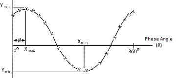
From this force history, the maximum and minimum forces are calculated by fitting the highest and lowest points. Then:
 | (15–104) |
 | (15–105) |
 | (15–106) |
so that  is the coefficient on the real load vector and
  is the coefficient on the imaginary load vector.