3-D 20-Node
Thermal Solid
SOLID279 Element Description
SOLID279 is a higher order 3-D 20-node solid element that exhibits quadratic thermal behavior. The element is defined by 20 nodes with a temperature degree of freedom at each node.
SOLID279 is available in these forms:
Homogeneous Thermal Solid (KEYOPT(3) = 0, the default) -- See "SOLID279 Homogeneous Thermal Solid Element Description".
Layered Thermal Solid (KEYOPT(3) = 1), or Layered Thermal Solid with through-the-thickness degrees of freedom (KEYOPT(3) = 2) -- See "SOLID279 Layered Thermal Solid Element Description".
A lower-order version of the SOLID279 element is SOLID278.
SOLID279 Homogeneous Thermal Solid Element Description
SOLID279 homogeneous Thermal Solid is well suited to modeling irregular meshes (such as those produced by various CAD/CAM systems). The element may have any spatial orientation.
Various printout options are available. See SOLID279 in the Mechanical APDL Theory Reference for more details.

SOLID279 Homogeneous Thermal Solid Input Data
The geometry, node locations, and the element coordinate system for this element are shown in Figure 279.1: SOLID279 Homogeneous Thermal Solid Geometry. A prism-shaped element may be formed by defining the same node numbers for nodes K, L, and S; nodes A and B; and nodes O, P, and W. A tetrahedral-shaped element and a pyramid-shaped element may also be formed as shown in Figure 279.1: SOLID279 Homogeneous Thermal Solid Geometry. SOLID278 is a similar element, without mid-side nodes.
In addition to the nodes, the element input data includes the anisotropic material properties. Anisotropic material directions correspond to the element coordinate directions. The element coordinate system orientation is as described in Coordinate Systems.
As described in Coordinate Systems, you can use ESYS to orient the material properties and the temperature gradient and heat flux output. Use RSYS to choose output that follows the material coordinate system or the global coordinate system.
Orthotropic material directions correspond to the element coordinate directions. The element coordinate system orientation is as described in Coordinate Systems. Specific heat and density are ignored for steady-state solutions. Properties not input default as described in the Material Reference.
Element loads are described in Nodal Loading. Convection or heat flux (but not both) and radiation may be input as surface loads at the element faces as shown by the circled numbers on Figure 279.1: SOLID279 Homogeneous Thermal Solid Geometry. Heat generation rates may be input as element body loads at the nodes. If the node I heat generation rate HG(I) is input, and all others are unspecified, they default to HG(I). If all corner node heat generation rates are specified, each midside node heat generation rate defaults to the average heat generation rate of its adjacent corner nodes.
The following table summarizes the element input. Element Input provides a general description of element input.
SOLID279 Homogeneous Thermal Solid Input Summary
- Nodes
I, J, K, L, M, N, O, P, Q, R, S, T, U, V, W, X, Y, Z, A, B
- Degrees of Freedom
TEMP
- Real Constants
None
- Material Properties
TB command: See Element Support for Material Models for this element. MP command: KXX, KYY, KZZ, DENS, C - Surface Loads
- Convection or Heat Flux (but not both) and Radiation (using Lab = RDSF) --
face 1 (J-I-L-K), face 2 (I-J-N-M), face 3 (J-K-O-N), face 4 (K-L-P-O), face 5 (L-I-M-P), face 6 (M-N-O-P)
- Body Loads
- Special Features
Birth and death Initial state - KEYOPT(3)
Layer construction:
- 0 --
Homogeneous Solid (default) -- Nonlayered
- KEYOPT(9)
Element-level matrix form:
- 0 --
Symmetric (default)
- 1 --
Nonsymmetric
SOLID279 Homogeneous Thermal Solid Output Data
The solution output associated with the element is in two forms:
Nodal temperatures included in the overall nodal solution
Additional element output as shown in Table 279.1: SOLID279 Element Output Definitions
Output temperatures may be read by structural solid elements (such as SOLID186) via the LDREAD,TEMP command.

The element heat flux directions are parallel to the element coordinate system.
A general description of solution output is given in Solution Output. See the Basic Analysis Guide for ways to view results.
The Element Output Definitions table uses the following notation:
A colon (:) in the Name column indicates that the item can be accessed by the Component Name method (ETABLE, ESOL). The O column indicates the availability of the items in the file Jobname.OUT. The R column indicates the availability of the items in the results file.
In either the O or R columns, “Y” indicates that the item is always available, a number refers to a table footnote that describes when the item is conditionally available, and “-” indicates that the item is not available.
Table 279.1: SOLID279 Element Output Definitions
| Label | Definition | O | R |
|---|---|---|---|
| EL | Element Number | Y | Y |
| NODES | Nodes - I, J, K, L, M, N, O, P | Y | Y |
| MAT | Material number | Y | Y |
| VOLU: | Volume | Y | Y |
| XC, YC, ZC | Location where results are reported | Y | 2 |
| HGEN | Heat generations HG(I), HG(J), HG(K), HG(L), HG(M), HG(N), HG(O), HG(P), HG(Q), ..., HG(Z), HG(A), HG(B) | Y | - |
| TG:X, Y, Z | Thermal gradient components | Y | Y |
| TF:X, Y, Z | Thermal flux (heat flow rate/cross-sectional area) components | Y | Y |
| FACE | Face label | 1 | - |
| NODES | Corner nodes on this face | 1 | - |
| AREA | Face area | 1 | 1 |
| HFILM | Film coefficient | 1 | - |
| TAVG | Average face temperature | 1 | 1 |
| TBULK | Fluid bulk temperature | 1 | - |
| HEAT RATE | Heat flow rate across face by convection | 1 | 1 |
| HEAT RATE/AREA | Heat flow rate per unit area across face by convection | 1 | - |
| HFLUX | Heat flux at each node of face | 1 | - |
| HFAVG | Average film coefficient of the face | - | 1 |
| TBAVG | Average face bulk temperature | - | 1 |
| HFLXAVG | Heat flow rate per unit area across face caused by input heat flux | - | 1 |
Available only at centroid as a *GET item.
Table 279.2: SOLID279 Item and Sequence Numbers lists output available through ETABLE using the Sequence Number method. See The General Postprocessor (POST1) in the Basic Analysis Guide and The Item and Sequence Number Table in this document for more information. The following notation is used in Table 279.2: SOLID279 Item and Sequence Numbers:
- Name
output quantity as defined in Table 279.1: SOLID279 Element Output Definitions
- Item
predetermined Item label for ETABLE
- FCn
sequence number for solution items for element Face n
SOLID279 homogeneous Thermal Solid Assumptions and Restrictions
The element must not have a zero volume. This occurs most frequently when the element is not numbered properly.
Elements may be numbered either as shown in Figure 279.1: SOLID279 Homogeneous Thermal Solid Geometry or may have the planes IJKL and MNOP interchanged.
The condensed face of a prism-shaped element should not be defined as a convection face.
The specific heat is evaluated at each integration point to allow for abrupt changes (such as melting) within a coarse grid of elements.
If the thermal element is to be replaced by a SOLID186 structural element with surface stresses requested, the thermal element should be oriented such that face IJNM and/or face KLPO is a free surface.
A free surface of the element (i.e., not adjacent to another element and not subjected to a boundary constraint) is assumed to be adiabatic.
Thermal transients having a fine integration time step and a severe thermal gradient at the surface will also require a fine mesh at the surface.
An edge with a removed midside node implies that the temperature varies linearly, rather than parabolically, along that edge.
See Quadratic Elements (Midside Nodes) in the Modeling and Meshing Guide for more information about the use of midside nodes.
For transient solutions using the THOPT,QUASI option, the program removes the midside nodes from any face with a convection load. A temperature solution is not available for them. Do not use the midside nodes on these faces in constraint equations or with contact. If you use these faces for those situations, remove the midside nodes first.
Degeneration to the form of pyramid should be used with caution.
The element sizes, when degenerated, should be small in order to minimize the field gradients.
Pyramid elements are best used as filler elements or in meshing transition zones.
This element is available in layered form. See "SOLID279 Layered Thermal Solid Assumptions and Restrictions".
SOLID279 Layered Thermal Solid Element Description
Use SOLID279 Layered Thermal Solid
to model heat conduction in layered thick shells or solids. The layered
section definition is given by section (SECxxx) commands. A prism degeneration option is also available.
Figure 279.3: SOLID279 Layered Thermal Solid Geometry

xo = Element x-axis if ESYS is not specified.
x = Element x-axis if ESYS is specified.
SOLID279 Layered Thermal Solid Input Data
The geometry, node locations, and the element coordinate system for this element are shown in Figure 279.3: SOLID279 Layered Thermal Solid Geometry. A prism-shaped element may be formed by defining the same node numbers for nodes K, L, and S; nodes A and B; and nodes O, P, and W.
In addition to the nodes, the element input data includes the anisotropic material properties. Anisotropic material directions correspond to the layer coordinate directions which are based on the element coordinate system. The element coordinate system follows the shell convention where the z axis is normal to the surface of the shell. The nodal ordering must follow the convention that I-J-K-L and M-N-O-P element faces represent the bottom and top shell surfaces, respectively. You can change the orientation within the plane of the layers via the ESYS command in the same way that you would for shell elements (as described in Coordinate Systems). To achieve the correct nodal ordering for a volume mapped (hexahedron) mesh, you can use the VEORIENT command to specify the desired volume orientation before executing the VMESH command. Alternatively, you can use the EORIENT command after automatic meshing to reorient the elements to be in line with the orientation of another element, or to be as parallel as possible to a defined ESYS axis.
Layered Section Definition Using Section Commands
You can associate SOLID279 Layered
Thermal Solid with a shell section (SECTYPE). The
layered composite specifications (including layer thickness, material,
orientation, and number of integration points through the thickness
of the layer) are specified via shell section (SECxxx) commands. You can use the shell section commands even with a single-layered
element. ANSYS obtains the actual layer thicknesses used for element
calculations by scaling the input layer thickness so that they are
consistent with the thickness between the nodes.
You can designate the number of integration points (1, 3, 5, 7, or 9) located through the thickness of each layer. Two points are located on the top and bottom surfaces respectively and the remaining points are distributed equal distance between the two points. The element requires at least two points through the entire thickness. When no shell section definition is provided, the element is treated as single-layered and uses two integration points through the thickness.
SOLID279 Layered Thermal Solid does not support real constant input for defining layer sections.
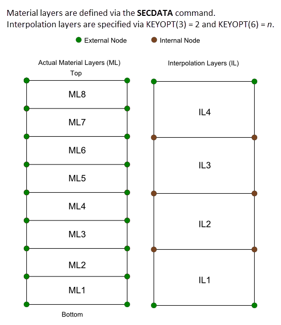
SOLID279 Layered
Thermal Solid has an option for through-the-thickness degrees of freedom
(KEYOPT(3) = 2). As shown in Figure 279.4: Understanding Interpolation Layers,
the option works by creating a specified number of material layers
(defined via the SECDATA command) per interpolation
layer (KEYOPT(6) = n). Each interpolation
layer has four internal nodes,
one on each face. Actual midside nodes (Y, Z, A, and B) on the material layers are ignored. KEYOPT(3)
= 2 offers greater accuracy than KEYOPT(3) = 1 but is more computationally
intensive; the more material layers specified per interpolation layer,
the greater the accuracy and computational cost.
Other Input
The default orientation for this element has the S1 (shell surface coordinate) axis aligned with the first parametric direction of the element at the center of the element and is shown as xo in Figure 279.3: SOLID279 Layered Thermal Solid Geometry.
The default first surface direction S1 can be reoriented in the element reference plane (as shown in Figure 279.3: SOLID279 Layered Thermal Solid Geometry) via the ESYS command. You can further rotate S1 by angle THETA (in degrees) for each layer via the SECDATA command to create layer-wise coordinate systems. See Coordinate Systems for details.
Orthotropic material directions correspond to the element coordinate directions. The element coordinate system orientation is as described in Coordinate Systems. Specific heat and density are ignored for steady-state solutions. Properties not input default as described in the Material Reference.
Element loads are described in Nodal Loading. Convection or heat flux (but not both) and radiation may be input as surface loads at the element faces as shown by the circled numbers on Figure 279.3: SOLID279 Layered Thermal Solid Geometry. Heat generation rates may be input as element body loads on a per layer basis. One heat generation value is applied to the entire layer. If the first layer heat generation rate HG(1) is input, and all others are unspecified, they default to HG(1).
As described in Coordinate Systems, you can use the ESYS command to orient the material properties and temperature gradient/heat flux output. Use RSYS to choose output that follows the material coordinate system or the global coordinate system.
The following table summarizes the element input. Element Input provides a general description of element input.
SOLID279 Layered Thermal Solid Input Summary
- Nodes
I, J, K, L, M, N, O, P, Q, R, S, T, U, V, W, X, Y, Z, A, B
- Degrees of Freedom
TEMP
- Real Constants
None
- Material Properties
TB command: See Element Support for Material Models for this element. MP command: KXX, KYY, KZZ, DENS, C - Surface Loads
- Convection or Heat Flux (but not both) and Radiation (using Lab = RDSF) --
face 1 (J-I-L-K), face 2 (I-J-N-M), face 3 (J-K-O-N), face 4 (K-L-P-O), face 5 (L-I-M-P), face 6 (M-N-O-P)
- Body Loads
- Heat Generations --
HG(1), HG(2), HG(3), . . . , HG(number of layers)
For the layered solid (KEYOPT(3) = 1 or 2), heat generation can be defined with the BFE command only.
- Special Features
- KEYOPT(3)
Layer construction:
- 1 --
Layered Solid
- 2 --
Layered Solid with through-the-thickness degrees of freedom
- KEYOPT(6)
Number of material layers (>= 1) per interpolation layer (valid only when KEYOPT(3) = 2):
- 1 --
Single layer (default)
n--Specified number
nof layers
- KEYOPT(8)
Material layer data storage:
- 0 --
Store data for bottom of bottom layer and top of top layer (default)
- 1 --
Store top and bottom data for all layers. (The volume of data may be considerable.)
- KEYOPT(9)
Element-level matrix form:
- 0 --
Symmetric (default)
- 1 --
Nonsymmetric
SOLID279 Layered Thermal Solid Output Data
The solution output associated with the element is in two forms:
Nodal temperatures included in the overall nodal solution
Additional element output as shown in Figure 279.5: SOLID279 Layered Thermal Solid Temperature Gradient/Heat Flux Output
Output temperatures may be read by structural solid elements (such as SOLID186) via the LDREAD,TEMP command.

The element heat flux directions are parallel to the layer coordinate system.
Convection heat flux is positive out of the element; applied heat flux is positive into the element.
The element output directions are parallel to the element coordinate system.
A general description of solution output is given in Solution Output. See the Basic Analysis Guide for ways to view results.
To see the temperature distribution through the thickness for this element, enter the POST1 postprocessor (/POST1), then issue /GRAPHICS,POWER and /ESHAPE,1 followed by PLESOL,BFE,TEMP
The Element Output Definitions table uses the following notation:
A colon (:) in the Name column indicates that the item can be accessed by the Component Name method (ETABLE, ESOL). The O column indicates the availability of the items in the file Jobname.OUT. The R column indicates the availability of the items in the results file.
In either the O or R columns, “Y” indicates that the item is always available, a number refers to a table footnote that describes when the item is conditionally available, and “-” indicates that the item is not available.
Table 279.3: SOLID279 Element Output Definitions
| Label | Definition | O | R |
|---|---|---|---|
| EL | Element Number | Y | Y |
| NODES | Nodes - I, J, K, L, M, N, O, P | Y | Y |
| MAT | Material number | Y | Y |
| VOLU: | Volume | Y | Y |
| XC, YC, ZC | Location where results are reported | Y | 2 |
| TG:X, Y, Z | Thermal gradient components | Y | Y |
| TF:X, Y, Z | Thermal flux (heat flow rate/cross-sectional area) components | Y | Y |
| FACE | Face label | 1 | - |
| NODES | Corner nodes on this face | 1 | - |
| AREA | Face area | 1 | 1 |
| HFILM | Film coefficient | 1 | - |
| TAVG | Average face temperature | 1 | 1 |
| TBULK | Fluid bulk temperature | 1 | - |
| HEAT RATE | Heat flow rate across face by convection | 1 | 1 |
| HEAT RATE/AREA | Heat flow rate per unit area across face by convection | 1 | - |
| HFLUX | Heat flux at each node of face | 1 | - |
| HFAVG | Average film coefficient of the face | - | 1 |
| TBAVG | Average face bulk temperature | - | 1 |
| HFLXAVG | Heat flow rate per unit area across face caused by input heat flux | - | 1 |
Available only at centroid as a *GET item.
Table 279.4: SOLID279 Item and Sequence Numbers lists output available via ETABLE using the Sequence Number method. See The General Postprocessor (POST1) in the Basic Analysis Guide and The Item and Sequence Number Table in this document for more information. The following notation is used in Table 279.4: SOLID279 Item and Sequence Numbers:
- Name
output quantity as defined in Table 279.3: SOLID279 Element Output Definitions
- Item
predetermined Item label for ETABLE
- FCn
sequence number for solution items for element Face n
SOLID279 Layered Thermal Solid Assumptions and Restrictions
The element must not have a zero volume. This occurs most frequently when the element is not numbered properly.
Do add or remove midside nodes (EMID) when KEYOPT(3) = 2.
Elements may be numbered either as shown in Figure 279.3: SOLID279 Layered Thermal Solid Geometry or may have the planes IJKL and MNOP interchanged.
The condensed face of a prism-shaped element should not be defined as a convection face.
The specific heat is evaluated at each integration point to allow for abrupt changes (such as melting) within a coarse grid of elements.
If the thermal element is to be replaced by a SOLID186 structural element with surface stresses requested, the thermal element should be oriented such that face IJNM and/or face KLPO is a free surface.
A free surface of the element (i.e., not adjacent to another element and not subjected to a boundary constraint) is assumed to be adiabatic.
Thermal transients having a fine integration time step and a severe thermal gradient at the surface will also require a fine mesh at the surface.
An edge with a removed midside node implies that the temperature varies linearly, rather than parabolically, along that edge.
For more information about using midside nodes, see Quadratic Elements (Midside Nodes) in the Modeling and Meshing Guide.
For transient solutions using the THOPT,QUASI option, the program removes the midside nodes from any face with a convection load. A temperature solution is not available for them. Do not use the midside nodes on these faces in constraint equations or with contact. If you use these faces for those situations, remove the midside nodes first.
This element is primarily intended for conveniently modeling the in-plane effects in layered thick shells or solids. The in-plane conductivity is the average of the individual layer conductivities. For complicated through-the-thickness behaviors, consider using one of the following:
Through-the-thickness degrees of freedom (KEYOPT(3) = 2).
Multiple layers of homogeneous (nonlayered) SOLID279 elements.
SHELL131, the layered shell with through-the-thickness degrees of freedom
When using this element with through-the-thickness degrees of freedom (KEYOPT(3) = 2), loads applied on layered faces are not applied to the through-the-thickness degrees of freedom (internal nodes).
SOLID279 Product Restrictions
When used in the product(s) listed below, the stated product-specific restrictions apply to this element in addition to the general assumptions and restrictions given in the previous section.
ANSYS Mechanical Pro
Layered solid (KEYOPT(3) = 1 or 2) is not available. KEYOPT(3) defaults to 0 and cannot be changed.
Birth and death is not available.
ANSYS Mechanical Premium
Birth and death is not available.