CONTA178

3-D Node-to-Node Contact

Product Restrictions

CONTA178 Element Description

CONTA178 represents contact and sliding between any two nodes of any types of elements. The element has two nodes with three degrees of freedom at each node with translations in the X, Y, and Z directions. It can also be used in 2-D and axisymmetric models by constraining the UZ degree of freedom. The element is capable of supporting compression in the contact normal direction and Coulomb friction in the tangential direction. User-defined friction with the USERFRIC subroutine and user-defined interaction with the USERINTER subroutine are also allowed. The element may be initially preloaded in the normal direction or it may be given a gap specification. A longitudinal damper option can also be included. See CONTA178 in the Mechanical APDL Theory Reference for more details about this element. Other contact elements, such as COMBIN40, are also available.

Figure 178.1: CONTA178 Geometry

CONTA178 Input Data

The geometry, node locations, and the coordinate system for this element are shown in the CONTA178 figure above. The element is defined by two nodes, an initial gap or interference (GAP), an initial element status (START), and damping coefficients CV1 and CV2. The orientation of the interface is defined by the node locations (I and J) or by a user specified contact normal direction. The interface is assumed to be perpendicular to the I-J line or to the specified gap direction. The element coordinate system has its origin at node I and the x-axis is directed toward node J or in the user specified gap direction. The interface is parallel to the element y-z plane. See Generating Contact Elements in the Contact Technology Guide for more information on generating elements automatically using the EINTF command.

To model proper momentum transfer and energy balance between contact and target surfaces, impact constraints should be used in transient dynamic analysis. See the description of KEYOPT(7) in the Input Summary and the contact element discussion in the Mechanical APDL Theory Reference for details.

Contact Algorithms

Four different contact algorithms can be selected:

Pure Lagrange multiplier method (KEYOPT(2) = 4)
Lagrange multiplier on contact normal and penalty on frictional (tangential) direction (KEYOPT(2) = 3)
Augmented Lagrange method (KEYOPT(2) = 0)
Pure Penalty method (KEYOPT(2) = 1)

The following sections outline these four algorithms.

Pure Lagrange Multiplier

The pure Lagrange multiplier method does not require contact stiffness FKN, FKS. Instead it requires chattering control parameters TOLN, FTOL, by which ANSYS assumes that the contact status remains unchanged. TOLN is the maximum allowable penetration and FTOL is the maximum allowable tensile contact force.

Note: A negative contact force occurs when the contact status is closed. A tensile contact force (positive) refers to a separation between the contact surfaces, but not necessarily an open contact status.

The behavior can be described as follows:

If the contact status from the previous iteration is open and the current calculated penetration is smaller than TOLN, then contact remains open. Otherwise the contact status switches to closed and another iteration is processed.
If the contact status from the previous iteration is closed and the current calculated contact force is positive, but smaller than FTOL, then contact remains closed. If the tensile contact force is larger than FTOL, then the contact status changes from closed to open and ANSYS continues to the next iteration.

ANSYS will provide reasonable defaults for TOLN and FTOL. Keep in mind the following when providing values for TOLN and FTOL:

A positive value is a scaling factor applied to the default values.
A negative value is used as an absolute value (which overrides the default).

The objective of TOLN and FTOL is to provide stability to models which exhibit contact chattering due to changing contact status. If the values you use for these tolerances are too small, the solution will require more iterations. However, if the values are too big it will affect the accuracy of the solution, since a certain amount of penetration or tensile contact force are allowed.

Theoretically, the pure Lagrange multiplier method enforces zero penetration when contact is closed and "zero slip" when sticking contact occurs. However the pure Lagrange multiplier method adds additional degrees of freedom to the model and requires additional iterations to stabilize contact conditions. This will increase the computational cost and may even lead to solution divergence if many contact points are oscillating between sticking and sliding conditions during iterations.

Lagrange Multiplier on Normal and Penalty on Tangent Plane

An alternative algorithm is the Lagrange multiplier method applied on the contact normal and the penalty method (tangential contact stiffness) on the frictional plane. This method only allows a very small amount of slip for a sticking contact condition. It requires chattering control parameters TOLN, FTOL as well as the maximum allowable elastic slip parameter SLTOL. Again, ANSYS provides default tolerance values which work well in most cases. You can override the default value for SLTOL by defining a scaling factor (positive value) or an absolute value (negative value). Based on the tolerance, current normal contact force, and friction coefficient, the tangential contact stiffness FKS can be obtained automatically. In a few cases, you can override FKS by defining a scaling factor (positive input) or absolute value (negative input). Use care when specifying values for SLTOL and FKS. If the value for SLTOL is too large and the value for FKS too small, too much elastic slip can occur. If the value for SLTOL is too small or the value for FKS too large, the problem may not converge.

Augmented Lagrange Method

The third contact algorithm is the augmented Lagrange method, which is basically the penalty method with additional penetration control. This method requires contact normal stiffness FKN, maximum allowable penetration TOLN, and maximum allowable slip SLTOL. FKS can be derived based on the maximum allowable slip SLTOL and the current normal contact force. ANSYS provides a default normal contact stiffness FKN which is based on the Young's modulus E and the size of the underlying elements. If Young's modulus E is not found, E = 1x10⁹ will be assumed.

You can override the default normal contact stiffness FKN by defining a scaling factor (positive input) or absolute value (negative input with unit force/length). If you specify a large value for TOLN, the augmented Lagrange method works as the penalty method. Use care when specifying values for FKN and TOLN. If the value for FKN is too small and the value for TOLN too large, too much penetration can occur. If the value for FKN is too large or the value for TOLN too small, the problem may not converge.

Penalty Method

The last algorithm is the pure penalty method. This method requires both contact normal and tangential stiffness values FKN, FKS. Real constants TOLN, FTOLN, and SLTOL are not used and penetration is no longer controlled in this method. Default FKN is provided as the one used in the augmented Lagrange method. The default FKS is given by MU x FKN. You can override the default values for FKN and FKS by inputting a scaling factor (positive input) or absolute value (negative input) for these real constants.

Contact Normal Definition

The contact normal direction is of primary importance in a contact analysis. By default [KEYOPT(5) = 0 and NX, NY, NZ = 0], ANSYS will calculate the contact normal direction based on the initial positions of the I and J nodes, such that a positive displacement (in the element coordinate system) of node J relative to node I opens the gap. However, you must specify the contact normal direction for any of the following conditions:

If nodes I and J have the same initial coordinates.
If the model has an initial interference condition in which the underlying elements' geometry overlaps.
If the initial open gap distance is very small.

In the above cases, the ordering of nodes I and J is critical. The correct contact normal usually points from node I toward node J unless contact is initially overlapped.

You can specify the contact normal by means of real constants NX, NY, NZ (direction cosines related to the global Cartesian system) or element KEYOPT(5). The following lists the various options for KEYOPT(5):

KEYOPT(5) = 0: The contact normal is either based on the real constant values of NX, NY, NZ or on node locations when NX, NY, NZ are not defined. For 2-D contact, NZ = 0.
KEYOPT(5) = 1 (2,3): The contact normal points in a direction which averages the direction cosines of the X (Y, Z) axis of the nodal coordinates on both nodes I and J. The direction cosines on nodes I and J should be very close. This option may be supported by the NORA and NORL commands, which rotate the X axis of the nodal coordinate system to point to the surface normal of solid models.
KEYOPT(5) = 4 (5,6): The contact normal points to X (Y, Z) of the element coordinate system issued by the ESYS command. If you use this option, make sure that the element coordinate system specified by ESYS is the Cartesian system. Otherwise, the global Cartesian system is assumed.

Note that the above discussion pertains to the unidirectional gap option (KEYOPT(1) = 0). For the definition of the contact normal for other gap options, see "Cylindrical Gap" and "Spherical Gap".

Contact Status

The initial gap defines the gap size (if positive) or the displacement interference (if negative). If KEYOPT(4) = 0, the default, the gap size can be automatically calculated from the GAP real constant and the node locations (projection of vector points from node I to J on the contact normal), that is, the gap size is determined from the additive effect of the geometric gap and the value of GAP.

If KEYOPT(4) = 1, the initial gap size is only based on real constant GAP (node locations are ignored).

By default KEYOPT(9) is set to 0, which means the initial gap size is applied in the first load step. To ramp the initial gap size with the first load step (to model initial interference problems, for example), set KEYOPT(9) = 1. Also, set KBC,0 and do not specify any external loads over the first load step.

The force deflection relationships for the contact element can be separated into the normal and tangential (sliding) directions. In the normal direction, when the normal force (FN) is negative, the contact status remains closed (STAT = 3 or 2). In the tangential direction, for FN < 0 and the absolute value of the tangential force (FS) less than μ|FN|, contact "sticks" (STAT = 3). For FN < 0 and FS = μ|FN|, sliding occurs (STAT = 2). As FN becomes positive, contact is broken (STAT = 1) and no force is transmitted (FN = 0, FS = 0).

The contact condition at the beginning of the first substep can be determined from the START parameter. The initial element status (START) is used to define the "previous" condition of the interface at the start of the first substep. This value overrides the condition implied by the interference specification and can be useful in anticipating the final interface configuration and reducing the number of iterations required for convergence. However, specifying unrealistic START values can sometimes degrade the convergence behavior.

If START = 0.0 or blank, the initial status of the element is determined from either the GAP value or the KEYOPT(4) setting. If START = 3.0, contact is initially closed and not sliding (μ ≠ 0), or sliding (if μ = 0.0). If START = 2.0, contact is initially closed and sliding. If START = 1.0, contact is initially open.

Friction

The only structural material property used is the interface coefficient of friction μ (MU). A zero value should be used for frictionless surfaces. Temperatures may be specified at the element nodes (via the BF command in a structural analysis or the D command in a coupled thermal-structural analysis). The coefficient of friction μ is evaluated at the average of the two node temperatures. The node I temperature T(I) defaults to TUNIF. The node J temperature defaults to T(I).

For analyses involving friction, using NROPT,UNSYM is useful (and, in fact, sometimes required if the coefficient of friction μ is > 0.2) for problems where the normal and tangential (sliding) motions are strongly coupled.

To define a coefficient of friction for isotropic friction that is dependent on temperature, time, normal pressure, sliding distance, or sliding relative velocity, use the TBFIELD command along with TB,FRIC. See Contact Friction in the Material Reference for more information.

Rigid Coulomb friction can be modeled with KEYOPT(10) = 7. In penalty-based methods, there is some elastic sliding present based on FKS. With the rigid Coulomb friction option, no sliding stiffness is used, so the element is always in a sliding state. See Rigid Coulomb Friction for details.

This element also supports user-defined friction. To implement a user-defined friction model, use the TB,FRIC command with TBOPT = USER to specify friction properties and write a USERFRIC subroutine to compute friction forces. See Writing Your Own Friction Law (USERFRIC) in the Mechanical APDL Contact Technology Guide for more information on how to use this feature. See also the Guide to User-Programmable Features in the Mechanical APDL Programmer's Reference for a detailed description of the USERFRIC subroutine.

In addition to the user-defined friction subroutine, the contact interaction subroutine USERINTER is available for user-defined interface interactions, including interactions in the normal and tangential directions as well coupled-field interactions. See Defining Your Own Contact Interaction (USERINTER) in the Mechanical APDL Contact Technology Guide for more information on how to use this feature. See also the Guide to User-Programmable Features in the Mechanical APDL Programmer's Reference for a detailed description of the USERINTER subroutine.

Cross-sectional Area

You may specify the contact area (defaults to 1.0) associated with this element by specifying real constant AREA. This area is used to compute the normal pressure and the tangential stress values. For axisymmetric problems, the area should be input on a full 360° basis.

Weak Spring

KEYOPT(3) can be used to specify a "weak spring" across an open or free sliding interface, which is useful for preventing rigid body motion that could occur in a static analysis. The weak spring stiffness is computed by multiplying the normal stiffness KN by a reduction factor if the real constant REDFACT is positive (which defaults to 1 x 10^-6). The weak spring stiffness can be overridden if REDFACT has a negative value. Set KEYOPT(3) = 1 to add weak spring stiffness only to the contact normal direction when contact is open. Set KEYOPT(3) = 2 to add weak spring stiffness to the contact normal direction for open contact and tangent plane for frictionless or open contact.

The weak spring only contributes to global stiffness, which prevents a "singularity" condition from occurring during the solution phase if KEYOPT(3) = 1,2. By setting KEYOPT(3) = 3,4, the weak spring will contribute both to the global stiffness and the internal nodal force which holds two separated nodes.

Note: The weak spring option should never be used in conjunction with either the no-separation or bonded contact options defined by KEYOPT(10).

Contact Behavior

Use KEYOPT(10) to model the following different contact surface behaviors:

KEYOPT(10) = 0: Models standard unilateral contact; that is, normal pressure equals zero if separation occurs.
KEYOPT(10) = 1: Models rough frictional contact where there is no sliding. This case corresponds to an infinite friction coefficient and ignores the material property input MU.
KEYOPT(10) = 2: Models no separation contact, in which two gap nodes are tied (although sliding is permitted) for the remainder of the analysis once contact is established.
KEYOPT(10) = 3: Models bonded contact, in which two gap nodes are bonded in all directions (once contact is established) for the remainder of the analysis.
KEYOPT(10) = 4: Models no separation contact, in which two gap nodes are always tied (sliding is permitted) throughout the analysis.
KEYOPT(10) = 5: Models bonded contact, in which two gap nodes are bonded in all directions throughout the analysis.
KEYOPT(10) = 6: Models bonded contact, in which two gap nodes that are initially in a closed state will remain closed and two gap nodes that are initially in an open state will remain open throughout the analysis.
KEYOPT(10) = 7: Models rigid Coulomb frictional contact in which sliding always occurs regardless of the magnitude of the normal contact force and the friction coefficient. Sticking contact never occurs and FKS is not used in this case. This option is useful for displacement-controlled problems or for certain dynamic problems where sliding dominates.

Cylindrical Gap

The cylindrical gap option (KEYOPT(1) = 1) is useful where the final contact normal is not fixed during the analysis, such as in the interaction between concentric pipes. With this option, you define the real constants NX, NY, NZ as the direction cosines of the cylindrical axis ( ) in the global Cartesian coordinate system. The contact normal direction lies in a cross section that is perpendicular to the cylindrical axis. The program measures the relative distance |XJ - XI| between the current position of node I and the current position of node J projected onto the cross section. NX, NY, NZ defaults to (0,0,1), which is the case for a 2-D circular gap. With the cylindrical gap option, KEYOPT(4) and KEYOPT(5) are ignored and node ordering can be arbitrary. Real constant GAP is no long referred as the initial gap size and a zero value is not allowed. The following explanation defines the model based on the sign of the GAP value.

Figure 178.2: CONTA178 - Cylindrical Gap

A positive GAP value models contact when one smaller cylinder inserted into another parallel larger cylinder. GAP is equal to the difference between the radii of the cylinders (|RJ - RI|) and it represents the maximum allowable distance projected on the cross-section. The contact constraint condition can be written as :
A negative GAP value models external contact between two parallel cylinders. GAP is equal to the sum of the radii of the cylinders (|RJ + RI|) and it represents the minimum allowable distance projected on the cross-section. The contact constraint condition can be written as:

Spherical Gap

The spherical gap option (KEYOPT(1) = 2) is useful when the final contact normal is not fixed during the analysis, such as in the interaction between two rigid spheres. With this spherical gap option, KEYOPT(4), KEYOPT(5), and real constants NX, NY, NZ are ignored. In addition, node ordering can be arbitrary. Real constant GAP is no longer referenced as the initial gap size, and a zero value is not allowed.

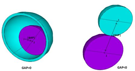
Figure 178.3: CONTA178 - Spherical Gap

The following explanation defines the model based on the sign of the GAP value:

A positive GAP value models contact when one smaller sphere is inside another large sphere. GAP is equal to the difference between the radii of the spheres (|RJ - RI|) and it represents the maximum allowable distance. The contact constraint condition can be written as:
A negative GAP value models external contact between two spheres. GAP is equal to the sum of the radii of the spheres (|RJ + RI|) and it represents the minimum allowable distance. The contact constraint condition can be written as:

Damper

The damping capability is only used for modal and transient analyses. By default, the damping capability is removed from the element. Damping is only active in the contact normal direction when contact is closed. The damping coefficient units are Force (Time/Length). For a 2-D axisymmetric analysis, the coefficient should be on a full 360° basis. The damping force is computed as , where C_v is the damping coefficient given by C_v = C_v1 + C_v2xV. V is the velocity calculated in the previous substep. The second damping coefficient (C_v2) is available to produce a nonlinear damping effect.

Modeling Thermal Contact

You can use the node-to-node contact element, in combination with thermal-structural coupled field solid elements or thermal elements, to model heat transfer that occurs between two contact nodes. To activate both the structural and thermal DOFs, set KEYOPT(6) = 1. To activate the thermal DOF only, set KEYOPT(6) = 2.

The contact normal direction must be specified, even in a purely thermal analysis (KEYOPT(6) = 2).

In the discussions below, note that the contacting area (AREA) is input as a real constant; it is not automatically calculated by the program.

Modeling Conduction

To take into account the conductive heat transfer between two contacting nodes, you need to specify the thermal contact conductance coefficient, which is real constant TCC.

The conduction function is defined as follows:

q(I) = -q(J) = TCC * AREA * (T(I) - T(J))

where:

q(I) = heat flow to node I (Heat/Time)

q(J) = heat flow to node J (Heat/Time)

AREA = cross sectional area (Length²) (defaults to 1)

TCC = thermal contact conductance coefficient (Heat/Length² * Time * Deg)

T(I) = temperature at node I (Deg)

T(J) = temperature at node J (Deg)

The TCC value is input through a real constant, which can be made a function of temperature [(T(I) + T(J))/2], pressure, time, penetration (positive input with GAP as a table parameter), and location by using the %tabname% option. If contact occurs, a small value of TCC yields a measured amount of imperfect contact and a temperature discontinuity across the two contacting nodes. For large values of TCC, the resulting temperature discontinuity tends to vanish, and perfect thermal contact is approached. When not in contact, however, it is assumed that no heat is transferred across the interface. To model contact conduction between two surfaces where a small gap exists, use KEYOPT(10) = 4 or 5 to define either the “bonded contact” or “no-separation contact” option.

Modeling Convection

The standard convection function is defined as follows:

q(I) = -q(J) = -CONV * AREA * (T(I) - T(J))

where:

CONV = Heat convection coefficient (Heat/Length² * Time * Deg))

To model convective heat transfer between two opening nodes, you must specify the heat convection coefficient CONV using the SFE command (with KVAL = 1 and CONV as a table parameter). CONV can be a constant value (only uniform is allowed) or a function of temperature [T(I) + T(J))/2], time, or location as specified through tabular input. If CONV is not defined through the SFE command, real constant TCC will be used instead only if tabular input or a user subroutine is used. TCC can be made a function of temperature [(T(I) + T(J))/2], pressure, time, gap (negative value input with GAP as a table parameter), and location by using the %tabname% option.

Modeling Radiation

The standard radiation function is defined as follows:

q(I) = -q(J) = -RDVF * EMIS * SBCT * AREA* [(T(I) + TOFFST)⁴ - (T(J)) + TOFFST)⁴]

where:

TOFFST = the temperature offset from absolute zero to zero (defined through the TOFFST command)

EMIS = surface emissivity (input as a material property)

SBCT = The Stefan-Boltzmann constant (input as a real constant). There is no default for SBCT; if it is not defined, the radiation effect is excluded. (BTU/Hr * in² * R⁴)

RDVF = The radiation view factor input as a real constant (defaults to 1). RDVF can be defined as a function of temperature, gap distance (negative value input with GAP as a table parameter), time, and location by using the %tabname% option.

Modeling Heat Generation Due to Friction

The standard frictional heat function is defined as follows:

q(I) = FHTG * FWGT * FDDIS
q(J) = FHTG * (1.0 - FWGT) * FDDIS

where:

FHTG = the fraction of frictionally dissipated energy converted into heat (defaults to 1.0). For an input of true zero, you must enter a very small value (for example, 1E-8). If you enter 0, the program interprets this input as the default value.

FWGT = the weight factor for the distribution of heat between node I and node J (defaults to 0.5)

FDDIS = frictional energy dissipation (Heat/Time)

In order to model heat generation due to frictionally dissipated energy, you would typically perform a coupled transient thermal-structural analysis. If inertia effects are negligible, you can turn off transient effects on structural DOFs by using the command TIMINT,STRUC,OFF. However, you should generally include transient effects on the thermal DOF.

In a steady-state coupled thermal-structural analysis, the friction-induced heat is still accounted for. The program computes the frictional energy dissipation as follows:

FDDIS = (total accumulated frictional energy)/(total time of the current load step)

In this case, the time of the current load step cannot be described as arbitrary. If you wish to neglect the friction-induced heat generation in the steady-state coupled thermal-structural analysis, use FHTG to specify a very small fraction of the frictionally dissipated energy (for example, FHTG = 1E-8).

Modeling External Heat Flux

You can apply an external flux through the SFE command. Only a uniform flux can be applied. The node J heat flux, HFLUX(J), defaults to the node I heat flux, HFLUX(I). The external heat flux is active only for opening contact.

The heat flow is defined as follows:

q(I) = q(J) = FLUX * AREA

where:

FLUX = applied heat flux, HFLUX(I)

Modeling Electric Contact

You can use the node-to-node contact element, in combination with thermal-electric elements and solid coupled field elements, to model electric current conduction between the two contacting nodes. You can also use the node-to-node contact element, in combination with piezoelectric and electrostatic elements, to model electric charge between the two contacting nodes.

KEYOPT(6) provides degree of freedom options for modeling electric contact. For combined structural/thermal/electric contact, set KEYOPT(6) = 3 to activate the structural, thermal, and electric current DOFs. For pure thermal/electric contact, set KEYOPT(6) = 4 to activate the thermal and electric current DOFs. For piezoelectric contact, set KEYOPT(6) = 5 to activate the structural and piezoelectric DOFs. For electrostatic contact, set KEYOPT(6) = 6 to activate the electrostatic DOF.

The contact normal direction must be specified, even in a purely electrical analysis (KEYOPT(6) = 6).

In the discussions below, note that the contacting area (AREA) is input as a real constant; it is not automatically calculated by the program.

Modeling Electric Conduction

To take into account the surface interaction for electric contact, you need to specify the electric contact conductance if you are using the electric current degree of freedom, or the electric contact capacitance if you are using the piezoelectric or electrostatic degrees of freedom. For either case, this parameter is specified through a real constant ECC.

The interaction between the two contacting surfaces is defined by:

J = ECC * AREA * (V(I) - V(J))

where:

J = current density for the electric potential (VOLT) degree of freedom (KEYOPT(6) = 3 or 4), or the electric charge density (KEYOPT(6) = 5, or 6)

V(I) and V(J) = voltages at node I and node J

ECC = electric contact conductance for the electric potential (VOLT) degree of freedom (KEYOPT(6) = 3 or 4), or the electric contact capacitance per unit area for (KEYOPT(6) = 5, or 6)

The ECC value is input through a real constant, which can be a function of temperature [(T(I) + T(J))/2], pressure (PRESSURE as a table parameter), penetration (positive value input with GAP as a table parameter), gap (negative value input with GAP as a table parameter), and time by using the %tabname% option. For the current conduction option, the electric contact conductance ECC has units of electric conductivity/length. For the piezoelectric and electrostatic options, the electric contact capacitance ECC has units of capacitance per unit area. If the “bonded contact” or “no-separation contact” option is set, contact interaction can occur between two nodes separated by a narrow gap.

Modeling Heat Dissipation Due to Electric Current

For electric current field analyses (KEYOPT(6) = 3 or 4), the heat dissipation at node I and node J due to electric current is given by:

q(I) = FHEG * FWGT * J * (V(I) - V(J))
q(J) = FHEG * (1.0 - FWGT) * J * (V(I) - V(J))

where:

FHEG = the fraction of electrically dissipated energy converted into heat (Joule heating). This value defaults to 1 and can be input as a real constant. For an input of true zero, you must enter a very small value (for example, 1E-8). If you enter 0, the program interprets this input as the default value.

J = the current density

FWGT = the weight factor for the contact heat dissipation between node I and node J (input as a real constant). FWGT is the same real constant used for frictional heat generation. By default, FWGT = 0.5. For an input of true zero, you must enter a very small value (for example, 1E-8). If you enter 0, the program interprets this input as the default value.

Defining Real Constants in Tabular Format

For certain real constants, you can define the real constants as a function of primary variables by using tabular input. Table 178.2: Real Constants and Corresponding Primary Variables for CONTA178 lists real constants that allow tabular input and their associated primary variables.

Use the *DIM command to dimension the table and identify the variables. You should follow the positive and negative convention for the real constant values. The possible primary variables used in tabular input are:

Time (TIME)

X location (X) in local/global coordinates

Y location (Y) in local/global coordinates

Z location (Z) in local/global coordinates

Temperature (TEMP degree of freedom)

Contact normal force (PRESSURE); specify positive index values for compression, negative index values for tension

Geometric contact gap/penetration (GAP); specify positive index values for penetration, negative index values for an open gap

Note that the primary variables X, Y, and Z represent the coordinates of the contact detection points. Coordinate system applicability is determined by the *DIM command.

When defining the tables, the primary variables must be in ascending order in the table indices (as in any table array).

When defining real constants via the R, RMORE, or RMODIF command, enclose the table name in % signs (e.g., %tabname%). For example, given a table named CNREAL1 that contains normal contact stiffness (FKN) values, you would issue a command similar to the following:

RMODIF,NSET,1,%CNREAL1%      ! NSET is the real constant set ID associated with the contact pair

For more information and examples of using table inputs, see TABLE Type Array Parameters in the ANSYS Parametric Design Language Guide; Applying Loads Using TABLE Type Array Parameters in the Basic Analysis Guide; and the *DIM command in the Command Reference.

Defining Real Constants via a User Subroutine

You can write a USERCNPROP subroutine to define your own real constants. The real constants that can be defined via this user subroutine are noted in Table 178.1: CONTA178 Real Constants. For additional details, see Defining Your Own Real Constant (USERCNPROP) in the Contact Technology Guide, and the description of USERCNPROP in the Programmer's Reference.

Monitoring Contact Status

By default, the program will not print out contact status and contact stiffness for each individual element. Use KEYOPT(12) = 1 to print out such information, which may help in solving problems that are difficult to converge.

See the Contact Technology Guide for a detailed discussion on contact and using the contact elements. Node-to-Node Contact discusses CONTA178 specifically, including the use of real constants and KEYOPTs.

A summary of the element input is given in "CONTA178 Input Summary". A general description of element input is given in Element Input.

CONTA178 Input Summary

Nodes

I, J

Degrees of Freedom

UX, UY, UZ (if KEYOPT(6) = 0)

UX, UY, UZ, TEMP (if KEYOPT(6) = 1)

TEMP (if KEYOPT(6) = 2)

UX, UY, UZ, TEMP, VOLT (if KEYOPT(6) = 3)

TEMP, VOLT (if KEYOPT(6) = 4)

UX, UY, UZ, VOLT (if KEYOPT(6) = 5)

VOLT (if KEYOPT(6) = 6)

Real Constants

FKN, GAP, START, FKS, REDFACT, NX,

NY, NZ, TOLN, FTOL, SLTOL, CV1,

CV2, COR, AREA, TCC, FHTG, SBCT

RDVF, FWGT, ECC, FHEG

See Table 178.1: CONTA178 Real Constants for a description of the real constants

Material Properties

TB command: See Element Support for Material Models for this element.

MP command: MU, EMIS, DMPR

Surface Loads

Convection, Face 1 (input with SFE command)

Heat Flux, Face 1 (I-J) (input with SFE command)

Body Loads

Temperatures - T(I), T(J)

Special Features

Isotropic friction

Linear perturbation

Nonlinear gap type

User-defined contact interaction

User-defined friction

KEYOPT(1)

Gap type:

0 --: Unidirectional gap
1 --: Cylindrical gap
2 --: Spherical gap

KEYOPT(2)

Contact algorithm:

0 --: Augmented Lagrange method (default)
1 --: Pure Penalty method
3 --: Lagrange multiplier on contact normal and penalty on tangent (uses U/P formulation for normal contact, non-U/P formulation for tangential contact)
4 --: Lagrange multiplier method

KEYOPT(3)

Weak Spring:

0 --: Not used
1 --: Acts across an open contact (only contributes to stiffness)
2 --: Acts across an open contact or free sliding plane (only contributes to stiffness)
3 --: Acts across an open contact (contributes to stiffness and internal force)
4 --: Acts across an open contact or free sliding plane (contributes to stiffness and force)

KEYOPT(4)

Gap size:

0 --: Gap size based on real constant GAP + initial node locations
1 --: Gap size based on real constant GAP (ignore node locations)

KEYOPT(5)

Basis for contact normal:

0 --: Node locations or real constants NX, NY, NZ
1 --: X - component of nodal coordinate system (averaging on two contact nodes)
2 --: Y - component of nodal coordinate system (averaging on two contact nodes)
3 --: Z - component of nodal coordinate system (averaging on two contact nodes)
4 --: X - component of defined element coordinate system (ESYS)
5 --: Y - component of defined element coordinate system (ESYS)
6 --: Z - component of defined element coordinate system (ESYS)

KEYOPT(6)

Selects degrees of freedom:

0 --: UX, UY, UZ
1 --: UX, UY, UZ, TEMP
2 --: TEMP
3 --: UX, UY, UZ, TEMP, VOLT
4 --: TEMP, VOLT
5 --: UX, UY, UZ, VOLT
6 --: VOLT

KEYOPT(7)

Element level time incrementation control / impact control:

0 --: No control
1 --: Change in contact predictions are made to maintain a reasonable time/load increment
2 --: Change in contact predictions are made to achieve the minimum time/load increment whenever a change in contact status occurs
4 --: Use impact constraints for standard or rough contact (KEYOPT(12) = 0 or 1) in a transient dynamic analysis with automatic adjustment of the time increment

KEYOPT(9)

Initial gap step size application:

0 --: Initial gap size is step applied
1 --: Initial gap size is ramped in the first load step

KEYOPT(10)

Behavior of contact surface:

0 --: Standard
1 --: Rough
2 --: No separation (sliding permitted)
3 --: Bonded
4 --: No separation (always)
5 --: Bonded (always)
6 --: Bonded (initial)
7 --: Rigid Coulomb friction (resisting force only if MU > 0.0)

KEYOPT(12)

Contact Status:

0 --: Does not print contact status
1 --: Monitor and print contact status, contact stiffness

Table 178.1: CONTA178 Real Constants

No.	Name	Description
1	FKN	Normal stiffness [1] [2]
2	GAP	Initial gap size [1]
3	START	Initial contact status
4	FKS	Sticking stiffness [1] [2]
5	REDFACT	KN/KS reduction factor
6	NX	Defined gap normal - X component
7	NY	Defined gap normal - Y component
8	NZ	Defined gap normal - Z component
9	TOLN	Penetration tolerance
10	FTOL	Maximum tensile contact force
11	SLTOL	Maximum elastic slip
12	CV1	Damping coefficient
13	CV2	Nonlinear damping coefficient
14	COR	Coefficient of restitution
15	AREA	Cross-sectional area (defaults to 1.0)
16	TCC	Thermal contact conductance [1] [2]
17	FHTG	Fraction of frictionally dissipation energy converted into heat
18	SBCT	Stefan-Boltzmann constant. There is no default for SBCT. If this real constant is not defined, the radiation effect is excluded. The Stefan-Boltzmann constant should correspond to the units of the FE model to be solved (e.g., 0.1190E-10 Btu/hr-in²-R⁴; 5.67E-8 W/m²-K⁴)
19	RDVF	Radiation view factor [1] [2]
20	FWGT	Heat distribution weighing factor
21	ECC	Electric contact conductance [1] [2]
22	FHEG	The fraction of Joule dissipation energy converted into heat

This real constant can be defined as a function of certain primary variables.
This real constant can be defined by the user subroutine USERCNPROP.F.

Table 178.2: Real Constants and Corresponding Primary Variables for CONTA178

Real Constants		TIME	Location (X,Y,Z)	TEMP	PRESSURE [1]	GAP [2]	%_CNPROP% [4]
Number	Name
1	FKN	x	x	x	x [3]	x	x
2	GAP	x	x	x	x	x	x
4	FKS	x	x	x	x	x	x
12	CV1	x	x	x	x	x	x
13	CV2	x	x	x	x	x	x
16	TCC	x	x	x	x	x	x
19	RDVF	x	x	x		x	x
21	ECC	x	x	x	x	x	x

Contact normal force via the primary variable PRESSURE. For PRESSURE index values, specify positive values for compression, negative value for tension.
Geometric contact gap/penetration via the primary variable GAP. For GAP index values, specify positive values for penetration, negative values for an open gap.
Contact normal force at the end of the previous iteration, if it exists.
Real constant can be defined via the user subroutine USERCNPROP.

CONTA178 Output Data

The solution output associated with the element is in two forms:

Nodal displacements included in the overall nodal solution.
Additional element output as shown in Element Output Definitions.

The value of USEP is determined from the normal displacement (UN), in the element x-direction, between the contact nodes at the end of a substep. This value is used in determining the normal force, FN. The values represented by UT(Y, Z) are the total translational displacements in the element y and z directions. The maximum value printed for the sliding force, FS, is μ|FN|. Sliding may occur in both the element y and z directions. STAT describes the status of the element at the end of a substep.

If STAT = 3, contact is closed and no sliding occurs
If STAT = 1, contact is open
If STAT = 2, node J slides relative to node I

For a frictionless surface (μ = 0.0), the converged element status is either STAT = 2 or 1.

The element coordinate system orientation angles α and β (shown in Figure 178.1: CONTA178 Geometry) are computed by the program from the node locations. These values are printed as ALPHA and BETA respectively. α ranges from 0° to 360° and β from -90° to +90°. Elements lying along the Z-axis are assigned values of α = 0°, β = ± 90°, respectively. Elements lying off the Z-axis have their coordinate system oriented as shown for the general α, β position.

Note: For α = 90°, β → 90°, the element coordinate system flips 90° about the Z-axis. The value of ANGLE represents the principal angle of the friction force in the element y-z plane. A general description of solution output is given in Element Solution. See the Basic Analysis Guide for ways to view results.

The Element Output Definitions table uses the following notation:

A colon (:) in the Name column indicates that the item can be accessed by the Component Name method (ETABLE, ESOL). The O column indicates the availability of the items in the file Jobname.OUT. The R column indicates the availability of the items in the results file.

In either the O or R columns, “Y” indicates that the item is always available, a number refers to a table footnote that describes when the item is conditionally available, and “-” indicates that the item is not available.

Table 178.3: CONTA178 Element Output Definitions

Name	Definition	O	R
EL	Element Number	Y	Y
NODES	Nodes - I, J	Y	Y
XC, YC, ZC	Location where results are reported	Y	3
TEMP	T(I), T(J)	Y	Y
USEP	Gap size (gap = negative value; penetration = positive value)	Y	Y
FN	Normal force (along I-J line)	Y	Y
STAT	Element status	1	1
OLDST	Old contact status	1	1
ALPHA, BETA	Element orientation angles	Y	Y
MU	Coefficient of friction	2	2
UT(Y, Z)	Displacement (node J - node I) in element y and z directions	2	2
FS(Y, Z)	Tangential (friction) force in element y and z directions	2	2
ANGLE	Principal angle of friction force in element y-z plane	2	2
AREA	Cross-sectional area	Y	Y
VELOC	Normal velocity used for damping calculation	Y	Y
DAMPF	Damping force	Y	Y
AUTY	Total sliding in y direction		Y
AUTZ	Total sliding in z direction		Y
ELSI	Total equivalent elastic slip distance		Y
PLSI	Total (accumulated) equivalent plastic slip due to frictional sliding		Y
TEMP1	Temperature at node I	Y	Y
TEMP2	Temperature at node J	Y	Y
TCC	Conductance coefficient	Y	Y
CONV	Convection coefficient	Y	Y
RAC	Radiation coefficient	Y	Y
HFLUX1	Applied heat flux at node I	Y	Y
HFLUX2	Applied heat flux at node J	Y	Y
FLUX1	Total heat flow at node I	Y	Y
FLUX2	Total heat flow at node J	Y	Y
FDDIS	Frictional energy dissipation	Y	Y
FXCV	Heat flow due to convection	Y	Y
FXRD	Heat flow due to radiation	Y	Y
FXCD	Heat flow due to conductance	Y	Y
ECC	Electric contact conductance (for electric current DOF), or electric contact capacitance per unit area (for piezoelectric or electrostatic DOF)	Y	Y
VOLT1	Voltage at node I	Y	Y
VOLT2	Voltage at node J	Y	Y
HJOU	Contact power/area	Y	Y
CCONT	Contact charge density (charge/area)	Y	Y
JCONT	Contact current density (current/area)	Y	Y

If the value of STAT is:
1 - Open contact
2 - Sliding contact
3 - Sticking contact (no sliding)
If MU>0.0
Available only at centroid as a *GET item.

Table 178.4: CONTA178 Item and Sequence Numbers lists output available through the ETABLE command using the Sequence Number method. See The General Postprocessor (POST1) in the Basic Analysis Guide for more information. The following notation is used in Table 178.4: CONTA178 Item and Sequence Numbers :

Name: output quantity as defined in the Element Output Definition
Item: predetermined Item label for ETABLE command
E: sequence number for single-valued or constant element data

Table 178.4: CONTA178 Item and Sequence Numbers

Output Quantity Name	ETABLE and ESOL Command Input
Output Quantity Name	Item	E
FN	SMISC	1
FSY	SMISC	2
FSZ	SMISC	3
FLUX1	SMISC	4
FLUX2	SMISC	5
FDDIS	SMISC	6
HFLUX1	SMISC	7
HFLUX2	SMISC	8
FXCV	SMISC	9
FXRD	SMISC	10
FXCD	SMISC	11
HJOU	SMISC	12
CCONT	SMISC	13
JCONT	SMISC	13
STAT	NMISC	1
OLDST	NMISC	2
USEP	NMISC	3
ALPHA	NMISC	4
BETA	NMISC	5
UTY	NMISC	6
UTZ	NMISC	7
MU	NMISC	8
ANGLE	NMISC	9
KN	NMISC	10
KS	NMISC	11
TOLN	NMISC	12
FTOL	NMISC	13
SLTOL	NMISC	14
ELSI	NMISC	15
PLSI	NMISC	16
AREA	NMISC	17
VELOC	NMISC	18
DAMPF	NMISC	19
AUTY	NMISC	20
AUTZ	NMISC	21
TEMP1	NMISC	22
TEMP2	NMISC	23
CONV	NMISC	24
RAC	NMISC	25
TCC	NMISC	26
ECC	NMISC	27
VOLT1	NMISC	28
VOLT2	NMISC	29

You can list contact results through several POST1 postprocessor commands. The contact specific items for the PRNSOL and PRESOL commands are listed below:

STAT	Contact status
PENE	Contact penetration
PRES	Contact force
SFRIC	Contact tangential force
STOT	Total contact tangential force
SLIDE	Contact sliding distance
GAP	Contact gap distance
FLUX	Total heat flow at contact node

CONTA178 Assumptions and Restrictions

The element operates bilinearly only in static and nonlinear transient dynamic analyses. If used in other analysis types, the element maintains its initial status throughout the analysis.
The element is nonlinear and requires an iterative solution.
Nonconverged substeps are not in equilibrium.
Unless the contact normal direction is specified by (NX, NY, NZ) or KEYOPT(5), nodes I and J must not be coincident or overlapped since the nodal locations define the interface orientation. In this case the node ordering is not an issue. On the other hand, if the contact normal is not defined by nodal locations, the node ordering is critical. Use /PSYMB, ESYS to verify the contact normal and use EINTF,,,REVE to reverse the normal if wrong ordering is detected. To determine which side of the interface contains the nodes, use ESEL,,ENAM,,178 and then NSLE,,POS,1.
The element maintains its original orientation in either a small or a large deflection analysis unless the cylindrical gap option is used.
For real constants FKN, REDFACT, TOLN, FTOL, SLTOL and FKS, you can specify either a positive or negative value. ANSYS interprets a positive value as a scaling factor and interprets a negative value as the absolute value. These real constants can be changed between load steps or during restart stages.
The Lagrange multiplier methods introduce zero diagonal terms in the stiffness matrix. The PCG solver may encounter precondition matrix singularity. The Lagrange multiplier methods often overconstrain the model if boundary conditions, coupling, and constraint equations applied on the contact nodes overlay the contact constraints. Chattering is most likely to occur due to change of contact status, typically for contact impact problems. The Lagrange multipliers also introduce more degrees of freedom which may result in spurious modes for modal and linear eigenvalue bucking analysis. Therefore, the augmented Lagrange method option is the best choice for: PCG iterative solver, transient analysis for impact problems, modal, and eigenvalue bucking analysis.
The element may not be deactivated with the EKILL command.

CONTA178 Product Restrictions

When used in the product(s) listed below, the stated product-specific restrictions apply to this element in addition to the general assumptions and restrictions given in the previous section.

ANSYS Mechanical Pro

User-defined contact is not available.
User-defined friction is not available.
Linear perturbation is not available.

ANSYS Mechanical Premium

User-defined contact is not available.
User-defined friction is not available.