The following topics are available in this section:
The following acoustic boundary condition topics are available:
For Dirichlet or Neumann boundary conditions, i.e., on a sound-soft boundary with p =
p0 (input as PRES on the D command) or on a
sound-hard boundary with  , the surface integration will be eliminated.
The Robin boundary condition on impedance boundary ΓZ is given by:
 | (8–34) |
where:
| vn,F = normal velocity of fluid particle on the boundary |
| vn,S = normal velocity of structure surface |
| Y = boundary admittance |
| Z (boundary impedance) = 1/Y (Z is input as IMPD on the SF command) |
Substituting Equation 8–34 into Equation 8–10 yields:
 | (8–35) |
For simplicity, the inviscid fluid will be investigated. The matrix forms in Equation 8–33 are rewritten as:
 | (8–36) |
 | (8–37) |
In acoustic design, the attenuation coefficient (i.e., the absorption coefficient) is used to define the absorption properties of the material. The attenuation coefficient is the ratio of the absorbed sound power density to the incident sound power density. The ratio is expressed as follows:
 | (8–38) |
where:

|

|
Because the module of reflection coefficient is given as  , the equivalent impedance (assumed Im(z)=0) of the attenuating material
is expressed as:
, the equivalent impedance (assumed Im(z)=0) of the attenuating material
is expressed as:
 | (8–39) |
where:
z0 = ρ0 c 0 = sound impedance
The impedance value of the Robin boundary condition can be defined by the sound impedance z0 = ρ0 c 0 (input as INF on the SF command), the attenuation coefficient (input as CONV on the SF command), or the general complex impedance (admittance the for modal analysis) (input as IMPD on the SF command). The Robin boundary condition can be used for the harmonic response or modal analysis.
The Floquet principle is satisfied when the acoustic wave propagates in a periodic
structure (input as Lab = FPBC on the BF
command or Label = PLAN on the APORT command
for plane wave incidence):
 | (8–40) |
where:
 = period of infinite periodic structure = period of infinite periodic structure |
 = complex propagating constant ( = complex propagating constant ( ); );  = attenuation constant; = attenuation constant;  = phase constant = phase constant |
A modified eigenvalue matrix equation solves the phase shift  as eigenvalues for acoustic elements if the phase shift is not equal to
0 or
as eigenvalues for acoustic elements if the phase shift is not equal to
0 or  :
:
 | (8–41) |
where:
 ( ( and and  are defined in Equation 8–33) are defined in Equation 8–33) |
 = the internal nodes = the internal nodes |
 = the master nodes for coupled master/slave nodes on the
boundary = the master nodes for coupled master/slave nodes on the
boundary |
 = slave nodes for coupled master/slave nodes on the
boundary = slave nodes for coupled master/slave nodes on the
boundary |
 as eigenvalue as eigenvalue |
Exterior structural acoustics problems typically involve a structure submerged in an infinite, homogeneous, inviscid fluid. For a source-free and inviscid fluid, Equation 8–5 is simplified as follows:
 | (8–42) |
where:

The pressure wave must satisfy the Sommerfeld radiation condition (which states that the waves generated within the fluid are outgoing) at infinity. This is expressed as:
 | (8–43) |
where:
| r = distance from the origin |
| d = dimensionality of the problem (i.e., d =3 or d =2 if Ω+ is 3-D or 2-D, respectively) |
A primary difficulty encountered when using finite elements to model an infinite medium arises from the need to satisfy the Sommerfeld radiation condition, as expressed in Equation 8–43. A typical approach to this problem involves truncating the unbounded domain Ω+ by introducing an absorbing (artificial) boundary Γa at some distance from the structure (Equation 8–5).
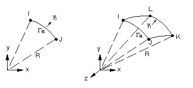
The homogeneous Helmholtz equation (Equation 8–42) is then solved in the annular region Ω+, which is bounded by the absorbing boundary Γa. For the resulting problem in Ω+ to be well-posed, an appropriate condition must be specified on Γa. To this end, the following second-order conditions are used on Γa (Kallivokas et al. [219]):
In two dimensions:
 | (8–44) |
where:
| n = outward normal to Γa |
| Pn = pressure derivative in the normal direction |
| Pλλ = pressure derivative along Γa |
| k = curvature of Γa |
| γ = stability parameter |
In three dimensions:
 | (8–45) |
where:
| n = outward normal |
| u and v = orthogonal curvilinear surface coordinates (e.g., the meridional and polar angles in spherical coordinates) |
| Pu, Pv = pressure derivatives in the Γa surface directions |
| H and K = mean and Gaussian curvature, respectively |
| E and G = usual coefficients of the first fundamental form |
Following a Galerkin based procedure, Equation 8–42 is multiplied by testing function w and integrated over the annular domain Ωf. By using the divergence theorem on the resulting equation it can be shown that:
 | (8–46) |
Upon discretization of Equation 8–46, the first term on the left hand side will yield the mass matrix of the fluid, while the second term will yield the stiffness matrix. The following finite element approximations for quantities on the absorbing boundary Γa placed at a radius R are introduced:
 | (8–47) |
where:
| {N} = vectors of shape functions |
| p, q(1), q(2) = unknown nodal values (p is output as degree of freedom PRES. q(1) and q(2) are solved for but not output.) |
Taking the nodal shape function as the testing function, the element stiffness and damping matrices can be further reduced. The two dimensional case is reduced to:
 | (8–48) |
 | (8–49) |
where:

|
| dl = arc-length differential |
These matrices are 6 x 6 in size, having 2 nodes per element with 3 degrees of freedom per node (p, q(1), q(2)). (See FLUID129 for details.)
The three dimensional case is reduced to:
 | (8–50) |
 | (8–51) |
where:

|

|

|
| ds = area differential |
For the three dimensional case, the surface element can be a quadratic or triangle element with corner and mid-nodes that have 2 degrees of freedom per node (p, q) (Barry et al. [218]). (See FLUID130 for details.)
For the axisymmetric case:
 | (8–52) |
 | (8–53) |
where:

|
| r = radius |
These matrices are 4x4 in size with 2 nodes per element and 2 degrees of freedom per node (p, q).
The local absorbing boundary conditions in this section are applicable to modal, harmonic response, or transient analyses.
Artificially matched layers are artificial anisotropic materials that absorb all incoming waves without any reflections, except for the grazing wave that parallels the artificially-matched-layers interface in the propagation direction. Artificially matched layers are currently constructed by the propagation of acoustic waves in the homogeneous isotropic media for harmonic response analysis (Zhao [407]).
The perfectly matched layers (PML) are located inside a cubic enclosure. The PML materials are specified in face, edge, and corner regions in a three-dimensional model.
In the frequency domain, the governing lossless and source-free momentum and conservation are given by:
 | (8–54) |
 | (8–55) |
The anisotropic PML material is assumed as follows:
 | (8–56) |
 | (8–57) |
where:
| [Λ] = diagonal tensor diag{sx, sy, sz}, and sx, sy, sz are complex constants. |
In order to satisfy the vector operation, the governing acoustic equations for PML are written as:
 | (8–58) |
 | (8–59) |
If the modified operator  is expressed as:
 | (8–60) |
Then the wave equation for a PML with a modified differential operator is expressed as:
 | (8–61) |
The interface between the PML and the real acoustic medium can be rendered reflectionless for all frequencies and angles of incidence of a wave propagating from the acoustic medium to the PML if the elements of [Λ] are defined as follows:
 | (8–62) |
where:
| σi = attenuation constant |
Multiplying sxsysz with Equation 8–61 results in the final wave equation needed to construct the PML:
 | (8–63) |
where:
| [Ψ] = diagonal tensor diag{sysz/sx, szsx/sy, sxsy/sz} |
By using the Galerkin method and setting the pressure to zero (input as PRES on the D command) on the backed boundary, the "weak" formulation of an acoustic pressure wave in PML is expressed as:
 | (8–64) |
Equation 8–64 can be written in matrix notation to produce the following discretized wave equation:
 | (8–65) |
where:

|

|

|
| SRe = real part of complex constant sxsysz |
| SIm = imaginary part of complex constant sxsysz |
| [ΨRe] = real part of complex tensor [Ψ] |
| [ΨIm] = imaginary part of complex tensor [Ψ] |
The PML material is defined using FLUID30, FLUID220, and FLUID221 elements with KEYOPT(4) = 1. Because the PML material is constructed in Cartesian coordinates, the edges of the 3-D PML region must be aligned with the axes of the global Cartesian coordinate system.
More than one 1-D PML region may exist in a finite element model. The PML element coordinate system (PSYS) uniquely identifies each PML region. A parabolic attenuation distribution is used to minimize numerical reflections in the PML. ANSYS, Inc. recommends using at least three PML element layers to obtain satisfactory accuracy. Some buffer elements between the PML region and objects should be utilized.
Because a PML acts as an infinite open domain, all boundary conditions and material properties need to be carried over into the PML region. The pressure must be set to zero (input as PRES on the D command) on the exterior surface of the PML, excluding Neumann boundaries (symmetric planes in the model). All types of excitation sources are prohibited in the PML region.
Refer to Artificially Matched Layers in the Mechanical APDL Acoustic Analysis Guide for more information about using PML.
Irregular perfectly matched layers (IPML) are located inside a convex enclosure. The IPML material is specified based on the local normal direction of the IPML interface. The pressure wave is assumed to propagate in the z'-direction of the local Cartesian coordinates (x', y', z'), which is set on the IPML interface by the program.
The wave equation for IPML with a modified differential operator is:
 | (8–66) |
The modified operator  is defined by:
 | (8–67) |
The complex IPML parameter is constructed by:
 | (8–68) |
Multiplying sz by Equation 8–66 results in the final wave equation for IPML as follows:
 | (8–69) |
where:
 = diagonal tensor diag{sz,
sz, 1/sz} = diagonal tensor diag{sz,
sz, 1/sz} |
The "weak" formulation of an acoustic pressure wave in IPML can be obtained with the
operator  and complex tensor in the local Cartesian coordinate system:
 | (8–70) |
The matrix notation for IPML is similar to Equation 8–65, except
for using the local operator and the complex tensor .
The IPML material is defined using FLUID30, FLUID220, and FLUID221 elements with KEYOPT(4) = 2. The IPML region must be a convex shape. The IPML is not related to any user-defined global or local coordinate system defined.
More than one 1-D IPML region may exist in a finite element model. A parabolic attenuation distribution is used to minimize numerical reflections in the IPML. ANSYS, Inc. recommends using at least three IPML element layers to obtain satisfactory accuracy and the uniform thickness of the IPML region. Some buffer elements between the IPML region and objects should be utilized.
All boundary conditions and material properties need to be carried over into the IPML region. The pressure must be set to zero (input as PRES on the D command) on the exterior surface of the IPML, excluding Neumann boundaries (rigid walls in the model). All types of excitation sources are prohibited in the IPML region. The program can automatically apply zero pressure to the exterior surface of the IPML region, but the rigid walls (the Neumann boundaries) have to be flagged (with the SF,,RIGW command), if they exist in the model.
Refer to Artificially Matched Layers in the Mechanical APDL Acoustic Analysis Guide for more information about using IPML.
Sound excitation sources are a fundamental part of an acoustic analysis. Various excitation sources, such as a monopole or plane wave can be imposed in simulations. The following methods can be used to introduce sound excitation sources:
Specified pressure or normal velocity on the domain boundary
Incident pressure applied on the exterior boundary (Robin boundary condition)
Incident pressure applied on the PML interface
Solve the wave equation with pure scattered pressure as a variable (Pure Scattered Pressure Formulation)
Analytic port modes in a duct:
Obliquely incident plane wave
Rectangular duct
Circular duct
Specified pressure (input as PRES on the D command) or normal velocity on the domain boundary offers a straightforward method to introduce the excitation source for harmonic response analysis (normal acceleration for transient analysis) (input as SHLD on the SF command) or the velocity for harmonic response analysis (acceleration for transient analysis) (input as EF on the BF command) (Equation 8–10) .
Mass source in the wave Equation 8–5 (input as JS on the BF command) can be used to introduce excitations for a pressure wave.
A point mass source is given by:
 | (8–71) |
where:
| Qp = magnitude of point mass source with unit [kg/s] |
| (xs, ys, zs) = source origin |
| δ = Dirac delta function |
A line mass source is given by:
 | (8–72) |
where:
| Ql = magnitude of line mass source with unit [kg/(ms)] |
A surface mass source is given by:
 | (8–73) |
where:
| Qs = magnitude of surface mass source with unit [kg/(m2s)] |
The volumetric mass source Q in Equation 8–8 has the unit [kg/(m3s)].
Depending on how the load is applied on the finite element,
the program will interpret the load as a point, line, surface, or
volumetric mass source. For a transient analysis, the mass source
rate ( ) in Equation 8–8 should
be defined.
) in Equation 8–8 should
be defined.
The various incident wave sources are defined using the AWAVE command for harmonic response analysis.
A time-harmonic incident planar wave (input as PLAN on the AWAVE command) is given by:
 | (8–74) |
where:
| Pinc,0= magnitude of incident planar wave |
| φ = initial phase angle of incident planar wave (usually ignored) |

|

|
The particle velocity is given by:
 | (8–75) |
A time-harmonic radiated monopole pressure (input as MONO on the AWAVE command) is introduced by:
 | (8–76) |
where:

|

|
| k = wave number |
If the normal velocity is along the  direction, the velocity of particle is given by:
 | (8–77) |
Assuming that the monopole is a pulsating sphere (r=a) with surface pressure pa, the pressure can be expressed as:
 | (8–78) |
If the normal velocity on the pulsating sphere surface is equal to va, the pressure is expressed as:
 | (8–79) |
Other applicable incident sources (Whitaker [[409]]) are also defined by the AWAVE command.
To apply the incident wave to the model, the splitting pressure should be introduced on the exterior excitation surface when the total pressure is solved by FEM. The total pressure consists of the incident pressure pinc and scattered pressure psc. This can be expressed as:
 | (8–80) |
For a planar wave, the incident wave and scattered wave can be written respectively as:
 | (8–81) |
 | (8–82) |
where:

|
Assuming the normal scattered wave vector is in the opposite direction of the normal incident wave vector, this can be expressed as:
 | (8–83) |
After substituting Equation 8–75 into the boundary integration of Equation 8–8, this can be expressed as:
 | (8–84) |
where:

|
The damping matrix and source vector in Equation 8–33 for lossless and source-free fluid with the planar incident wave on the exterior boundary is given by:
 | (8–85) |
 | (8–86) |
A similar procedure can be used for a spherical incident wave,
but the scattered wave is assumed to be a planar wave in the  direction. The damping matrix and source
vector in Equation 8–33 for lossless and source-free
fluid with the spherical incident wave on the exterior boundary is
given by:
direction. The damping matrix and source
vector in Equation 8–33 for lossless and source-free
fluid with the spherical incident wave on the exterior boundary is
given by:
 | (8–87) |
 | (8–88) |
If we assume that the incident wave perpendicularly projects on the transparent exterior surface of the model, the analogous derivation can be achieved with the Robin boundary condition (Equation 8–34), using the wave admittance Y0 as the impedance boundary. Since the incoming incident wave is propagating into the model, the Robin boundary condition is expressed as:
 | (8–89) |
where:

|
Assuming that the scattered wave has the same wave admittance as the incident wave, the Robin boundary condition for the outgoing scattered wave is expressed as:
 | (8–90) |
where:

|
Substituting Equation 8–89 into the boundary integration of Equation 8–8 and utilizing Equation 8–90 leads to:
 | (8–91) |
The damping matrix and source vector in Equation 8–33 for lossless and source-free fluid with the incident excitation on the impedance boundary is expressed as:
 | (8–92) |
 | (8–93) |
The above equations are useful for the analysis of the wave scattering and the pipe structure, respectively.
The planar scattered pressure wave propagating along the opposite direction of the incident wave is assumed to be on the exterior surface of the model, while the incident wave projects into the simulation domain from outside of the model. Obviously, this assumption leads to a numerical error once the non-planar scattered wave occurs. Hence, the PML is used to absorb the arbitrary scattered outgoing waves.
Assuming that the PML region is a scattered pressure region and that other regions are total pressure regions, the "weak" forms for the total pressure and the scattered pressure are respectively written as:
 | (8–94) |
In PML scattered pressure region:
 | (8–95) |
Total pressure can be split into scattered pressure and incident pressure on the interface between the general acoustic region and the PML region. This can be expressed as:
 | (8–96) |
The degrees of freedom on nodes with PML attributes are scattered pressure. The surface integration of scattered pressure on the interface will be cancelled out in Equation 8–94 and Equation 8–95. Assuming that the inside model is source free, the general matrix notation in the normal acoustic region, including the pressure on interface nodes, can be written as:
 | (8–97) |
Substituting Equation 8–96 into Equation 8–97 leads to the matrix equation for the interior total pressure and the interface scattered pressure, expressed as:
 | (8–98) |
The matrix equation for whole domain is expressed as:
 | (8–99) |
where:
 = complex stiffness matrix
for interior total pressure from Equation 8–98 = complex stiffness matrix
for interior total pressure from Equation 8–98
|
 = complex stiffness matrix
on interface from Equation 8–98 = complex stiffness matrix
on interface from Equation 8–98
|
 = complex stiffness matrix
for interface scattered pressure from Equation 8–98 = complex stiffness matrix
for interface scattered pressure from Equation 8–98
|
 = complex stiffness matrix
for PML interior scattered pressure from Equation 8–65 = complex stiffness matrix
for PML interior scattered pressure from Equation 8–65
|
| finc = complex source vector from Equation 8–98 |
The various analytic modes in a guided duct are defined using the APORT command for harmonic response analysis.
A time-harmonic incident planar wave (Label = PLAN on APORT) is given by:
 | (8–100) |
where:
 = complex initial pressure = complex initial pressure |
 = vector wave number = vector wave number |
 = position vector = position vector |
A mode existing in a rectangular duct (Label = RECT on
APORT) is given by:
 | (8–101) |
where:
 = width of duct = width of duct |
 = height of duct = height of duct |
 = propagating constant in z-direction = propagating constant in z-direction |
A mode existing in a circular duct (Label = CIRC on
APORT) is given by:
 | (8–102) |
where:
 = mth order
Bessel function of the first kind = mth order
Bessel function of the first kind |
 = nth zero of the derivative of the mth order Bessel function of the first kind = nth zero of the derivative of the mth order Bessel function of the first kind |
 = radius of the circular duct = radius of the circular duct |
A mode existing in a coaxial duct
(Label = COAX on APORT) is given
by:
 | (8–103) |
where:
 = coefficients determined by pressure and rigid wall boundary
condition at the inner radius r = a = coefficients determined by pressure and rigid wall boundary
condition at the inner radius r = a |
|
= mth order Bessel function of the first
kind |
 = mth order Bessel function of the second
kind = mth order Bessel function of the second
kind |
 = nth zero of the equation = nth zero of the equation 
|
|
= inner radius of the coaxial duct |
 = outer radius of the coaxial duct = outer radius of the coaxial duct |
The following topics are available in this section:
In non-uniform acoustic media the mass density and sound speed vary with the spatial position. Wave Equation 8–5 in lossless media is rewritten as:
 | (8–104) |
According to the ideal gas law, the equation of state and the speed of sound in an ideal gas are respectively expressed as:
 | (8–105) |
 | (8–106) |
where:

|
| CP = heat coefficient at a constant pressure per unit mass (input as C on the MP command) |
| CV = heat coefficient at a constant volume per unit mass (input as CVH on the MP command) |
| R = gas constant |
| T = temperature |
| Pstate = the absolute pressure of the gas measured in atmospheres |
Assuming density ρ0 (input as DENS on the MP command) and sound speed c0 (input as SONC on the MP command) at the reference temperature T0 (input on TREF command), and the reference static pressure (input as Psref on R command) the density and sound speed in media are cast as follows:
 | (8–107) |
 | (8–108) |
The spatial temperature is input as TEMP on BF command and the nodal static pressure is input as SPRE on the BF command.
Assuming that the skeleton of the perforated material is rigid, the perforated material can be approximated using the Johnson-Champoux-Allard equivalent fluid model, which uses the complex effective density and velocity (Allard [408]). The wave equation with complex effective density and velocity is given by:
 | (8–109) |
The effective density is given by:
 | (8–110) |
where:
| ω = angular frequency |
| σ = fluid resistivity |
| Φ = porosity |
| α ∞ = tortuosity |
| Λ = viscous characteristic length |
| ρ0 = density of fluid |
| η = dynamic (shear) viscosity |
The effective bulk modulus is given by:
 | (8–111) |
where:
| γ = specific heat ratio |
| P0 = static reference pressure (input as PSREF on the R command) |
| P rt=Cpη/κ = Prandtl number |
| Cp = specific heat |
| κ = thermal conductivity |
| Λ’ = thermal characteristic length |
The material coefficients used in the Johnson-Champoux-Allard model are input with the TBDATA command for the TB,PERF material as well as through MP commands.
The complex effective velocity is given by:
 | (8–112) |
The sound impedance is given by:
 | (8–113) |
The “weak” form of the Johnson-Champoux-Allard equivalent fluid model is given by:
 | (8–114) |
The matrix notation is expressed as:
 | (8–115) |
where:

|

|

|

|
The final matrix equation is expressed as:
 | (8–116) |
where:

|

|

|
Instead of inputting five parameters in the Johnson-Champoux-Allard model, only one parameter, fluid resistivity, is required in the Delany-Bazley and Miki models. In general, complex impedance is defined by:
 | (8–117) |
The complex propagation constant s is defined by
 | (8–118) |
where:
| R = resistance |
| X = reactance |
| α = attenuation constant |
| β = phase constant |
In both the Delany-Bazley and the Miki models, variables are approximated by the functions:
 | (8–119) |
 | (8–120) |
 | (8–121) |
 | (8–122) |
where:
| f = frequency |
| σ = fluid resistivity |
Coefficients are provided in the following table.
Table 8.1: Coefficients of the Approximation Functions for Delany-Bazley and Miki Models
| Coefficient | Delany-Bazley | Miki |
|---|---|---|
| a | 0.0497 | 0.0699 |
| b | -0.754 | -0.632 |
| c | 0.0758 | 0.107 |
| d | -0.732 | -0.632 |
| q | 0.169 | 0.160 |
| r | -0.618 | -0.618 |
| s | 0.0858 | 0.109 |
| t | -0.700 | -0.618 |
The proposed working range for the Delany-Bazley model is 0.01 <  < 1.00. The Miki model can be extended
to 0.01 <
< 1.00. The Miki model can be extended
to 0.01 <  .
.
The complex effective mass density and sound velocity in Equation 8–109 may be given by:
 | (8–123) |
 | (8–124) |
The Helmholtz equation with complex mass density and sound velocity is directly solved with the defined parameters.
The complex effective mass density and sound velocity are input with the TBDATA command for the TB,PERF material.
Analogous to Equation 8–34, the boundary condition across an impedance sheet in the acoustic domain is given by:
 | (8–125) |
where:

|

|

|

|
Assuming that the acoustic domain is divided into Ω+ and Ω- with the impedance sheet on the surface, substituting Equation 8–125 into Equation 8–10 casts the damping matrix as Equation 8–36. For a thin perforated layer, the sheet impedance (input as IMPD on the BF command) is given by:
 | (8–126) |
where:
| ZL = load impedance |
| d = thickness of perforated layer |
 = sound impedance
of the perforated material defined by Equation 8–113 = sound impedance
of the perforated material defined by Equation 8–113
|
 = complex wave
number of the perforated material (ceff is
defined by Equation 8–112) = complex wave
number of the perforated material (ceff is
defined by Equation 8–112) |
For a thin perforated material layer backed with a rigid wall, the impedance is given by:
 | (8–127) |
An acoustic waves propagating in viscous-thermal media have a complex propagating constant in the frequency domain. The attenuation of the acoustic wave is proportional to the shear and bulk viscosity and the thermal conduction coefficient of the media.
In a rigid-walled, bounded domain, the interaction between he acoustic movement and both the diffusion of heat and the diffusion of the shear wave leads to a reactive and absorbing process on the walls. The entropic and vortical perturbations diffuse into the rigid wall in a direction normal to the boundary and decay to zero depending on the thickness of the boundary layers. A hybrid numerical and analytic solution using the boundary layer impedance (BLI) model is proposed with the following assumptions ([415]):
The thicknesses of the boundary layers are much smaller than the dimensions of the numerical domain, while the pressure variation is constant over the boundary layers’ thicknesses.
The acoustic pressure is approximated by its zero expansion in the boundary layers and its flow is tangential to the wall.
Spatial variations of both velocity and temperature in the normal direction are much greater than spatial variations in the tangential directions.
The fundamental Helmholtz governing equation and boundary condition in the BLI model is given by:
 | (8–128) |
where:

|

|
| k0 = ω / c0 |
| lvh = lv+(γ-1)lh |
| kw = the transverse wavenumber |

|

|

|
| l’v = μ / (ρ0c0) |
| lh = λ / (ρ0c0Cp) |
| γ = Cp / Cv = the specific heat ratio |
| ω = the angular frequency |
| ρ0 = the mass density of the fluid |
| c0 = the sound speed of the fluid |
| μ = the dynamic viscosity |
| η = the bulk viscosity |
| λ = the thermal conductivity |
| Cp = the heat coefficient at constant pressure per unit mass |
| Cv = the heat coefficient at constant volume per unit mass |
The low reduced frequency (LRF) model is derived from simplified Navier-Stokes equations with the following assumptions ([416]):
The acoustic wavelength is much greater than the length scale of the geometry
The acoustic wavelength is much greater than the boundary layer thickness
The Helmholtz wave equation with modified density and bulk module for the LRF model is as follows:
 | (8–129) |
where:

|

|
| ρ0 = the mass density |
| K0 = the modified bulk module |
| l = the length scale |

|
| σ = Cpη / κ = Prandtl number |
| γ = specific heat ratio |
The viscous and thermal effects are taken into account by the function B(s/l) and n(sσ/l), respectively.
The analytic solution of both the functions B(s/l) and n(sσ/l) can be derived for three particular cases: thin layer, tube with rectangular cross-section, and tube with circular cross section.
A thin layer is specified by thickness h. The functions B(s/l) and n(sσ/l) are derived by:
 | (8–130) |
 | (8–131) |
where:

A tube with a rectangular cross-section is specified by width w and height h. The functions B(s/l) and n(sσ/l) are derived by:
 | (8–132) |
 | (8–133) |
where:

A tube with a circular cross section is specified by radius R. The functions B(s/l) and n(sσ/l) are derived by:
 | (8–134) |
 | (8–135) |
where:

| J0 = the zero-order Bessel function |
| J2 = the second-order Bessel function |