All continuum elements (2-D and 3-D solids, 3-D shells) are tested for acceptable shape as they are defined by the E, EGEN, AMESH, VMESH, or similar commands. This testing, described in the following sections, is performed by computing shape parameters (such as Jacobian ratio) which are functions of geometry, then comparing them to element shape limits whose default values are functions of element type and settings (but can be modified by the user on the SHPP command with Lab = MODIFY as described below). When defined, an element may generate no warnings, one or more warnings, or the element may be rejected with an error.
Some shape testing of 3-D solid elements (bricks [hexahedra], wedges, pyramids, and tetrahedra) is performed indirectly. Aspect ratio, parallel deviation, and maximum corner angle are computed for 3-D solid elements using the following steps:
Each of these 3 quantities is computed, as applicable, for each face of the element as though it were a quadrilateral or triangle in 3-D space, by the methods described in sections Aspect Ratio, Parallel Deviation, and Maximum Corner Angle.
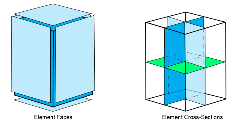
Because some types of 3-D solid element distortion are not revealed by examination of the faces, cross-sections through the solid are constructed. Then, each of the 3 quantities is computed, as applicable, for each cross-section as though it were a quadrilateral or triangle in 3-D space.
The metric for the element is assigned as the worst value computed for any face or cross-section.
A brick element has 6 quadrilateral faces and 3 quadrilateral cross-sections (Figure 12.1: Brick Element). The cross-sections are connected to midside nodes, or to edge midpoints where midside nodes are not defined.
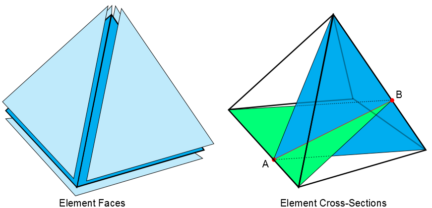
A pyramid element has 1 quadrilateral face and 4 triangle faces, as shown on the left side of Figure 12.2: Pyramid Element. The pyramid element has 8 triangle cross-sections, constructed in 4 pairs. One of the 4 pairs is shown on the right side of Figure 12.2: Pyramid Element.
For each pair, the closest points (A and B in the figure) between the lines containing a quadrilateral face edge and the right-ward opposite leg are found. The paired cross-sections are the triangle containing the quadrilateral face edge and point B and the triangle containing the right-ward opposite leg and point A. The remaining 6 cross-sections are found in a similar manner using the other 3 quadrilateral face edges and their corresponding right-ward legs.
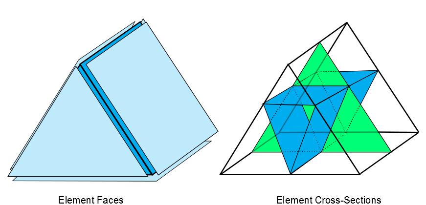
A wedge element has 3 quadrilateral and 2 triangle faces, and has 3 quadrilateral and 1 triangle cross-sections. As shown in Figure 12.3: Wedge Element, the cross-sections are connected to midside nodes, or to edge midpoints where midside nodes are not defined.
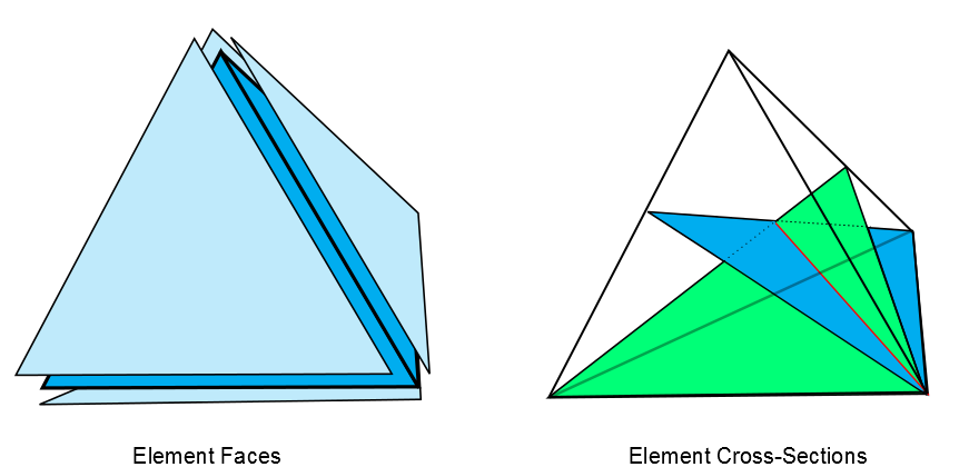
A tetrahedron element has 4 triangle faces and 6 triangle cross-sections (Figure 12.4: Tetrahedron Element). Each cross-section is the triangle containing one edge and the closest point on the line containing the opposite edge. Two of these cross-sections are shown on the right side of Figure 12.4: Tetrahedron Element.
An aspect ratio is computed and tested for all elements except Emag elements (see Table 12.1: Aspect Ratio Limits). Aspect ratio as a shape measure has been reported in finite element literature for decades (Robinson [121]) and is one of the easiest ones to understand. For triangles, equilateral triangles have an aspect ratio of 1 and the aspect ratio increases the more the triangle is stretched from an equilateral shape. For quadrilaterals, squares have an aspect ratio of 1 and the aspect ratio increases the more the square is stretched to an oblong shape. Some analysts want to be warned about high aspect ratio so they can verify that the creation of any stretched elements was intentional. Many other analysts routinely ignore it.
Unless elements are so stretched that numeric round off could become a factor (aspect ratio > 1000), aspect ratio alone has little correlation with analysis accuracy. Finite element meshes should be tailored to the physics of the given problem; i.e., fine in the direction of rapidly changing field gradients, relatively coarse in directions with less rapidly changing fields. Sometimes this calls for elements having aspect ratios of 10, 100, or in extreme cases 1000. (Examples include shell or thin coating analyses using solid elements, thermal shock “skin” stress analyses, and fluid boundary layer analyses.) Attempts to artificially restrict aspect ratio could compromise analysis quality in some cases.
For the benefit of computational efficiency, the aspect ratio of a triangle is computed based on the angle measures at the corner nodes rather than the height and width of the triangle. For the calculation, midside nodes are ignored and the triangle is treated as connecting nodes I, J, and K with straight lines:
For the angle θ, at node I, a quantity AMI is calculated as follows:
The quantity AMI is 1 when θ = 60°. As θ deviates from 60° in either direction, AMI increases (to a maximum of ∞ as θ nears 0° or 180°).
The quantity AM is calculated for each of the remaining nodes J and K.
A preliminary aspect ratio, ASPRAT, is calculated by averaging the three values of AM, then taking the square root:
Finally, the aspect ratio is modified to produce a distribution of values similar to those that would be produced if the aspect ratio were calculated directly from the height and width:


The best possible triangle aspect ratio, for an equilateral triangle, is 1. Larger aspect ratios are calculated as the triangle is stretched. Triangles having aspect ratios of 1 and 20 are shown in Figure 12.5: Aspect Ratios for Triangles.


The aspect ratio for a quadrilateral is computed by the following steps, using only the corner nodes of the element (Figure 12.6: Quadrilateral Aspect Ratio Calculation):
If the element is not flat, the nodes are projected onto a plane passing through the average of the corner locations and perpendicular to the average of the corner normals. The remaining steps are performed on these projected locations.
Two lines are constructed that bisect the opposing pairs of element edges and which meet at the element center. In general, these lines are not perpendicular to each other or to any of the element edges.
Rectangles are constructed centered about each of the 2 lines, with edges passing through the element edge midpoints. The aspect ratio of the quadrilateral is the ratio of a longer side to a shorter side of whichever rectangle is most stretched.
The best possible quadrilateral aspect ratio, for a square, is one. A quadrilateral having an aspect ratio of 20 is shown in Figure 12.7: Aspect Ratios for Quadrilaterals.

Table 12.1: Aspect Ratio Limits
| Command to modify | Type of Limit | Default | Why default is this tight | Why default is this loose |
|---|---|---|---|---|
| SHPP,MODIFY,1 | warning | 20 | Elements this stretched look to many users like they deserve warnings. |
Disturbance of analysis results has not been proven It is difficult to avoid warnings even with a limit of 20. |
| SHPP,MODIFY,2 | error | 106 | Informal testing has demonstrated solution error attributable to computer round off at aspect ratios of 1,000 to 100,000. |
Threshold of round off problems depends on what computer is being used. Valid analyses should not be blocked. |
Parallel deviation is computed and tested for all quadrilaterals or 3-D solid elements having quadrilateral faces or cross-sections, except Emag elements (see Table 12.2: Parallel Deviation Limits). Formal testing has demonstrated degradation of stress convergence in linear displacement quadrilaterals as opposite edges become less parallel to each other.
Parallel deviation is computed using the following steps:
Ignoring midside nodes, unit vectors are constructed in 3-D space along each element edge, adjusted for consistent direction, as demonstrated in Figure 12.8: Parallel Deviation Unit Vectors.
For each pair of opposite edges, the dot product of the unit vectors is computed, then the angle (in degrees) whose cosine is that dot product. The parallel deviation is the larger of these 2 angles. (In the illustration above, the dot product of the 2 horizontal unit vectors is 1, and acos (1) = 0°. The dot product of the 2 vertical vectors is 0.342, and acos (0.342) = 70°. Therefore, this element's parallel deviation is 70°.)
The best possible deviation, for a flat rectangle, is 0°. Figure 12.9: Parallel Deviations for Quadrilaterals shows quadrilaterals having deviations of 0°, 70°, 100°, 150°, and 170°.


Table 12.2: Parallel Deviation Limits
| Command to Modify | Type of Limit | Default | Why default is this tight | Why default is this loose |
|---|---|---|---|---|
| SHPP,MODIFY,11 | warning for elements without midside nodes | 70° | Testing has shown results are degraded by this much distortion | It is difficult to avoid warnings even with a limit of 70° |
| SHPP,MODIFY,12 | error for elements without midside nodes | 150° | Pushing the limit further does not seem prudent | Valid analyses should not be blocked. |
| SHPP,MODIFY,13 | warning for elements with midside nodes | 100° | Elements having deviations > 100° look like they deserve warnings. | Disturbance of analysis results for quadratic elements has not been proven. |
| SHPP,MODIFY,14 | error for elements with midside nodes | 170° | Pushing the limit further does not seem prudent | Valid analyses should not be blocked. |
Maximum corner angle is computed and tested for all except Emag elements (see Table 12.3: Maximum Corner Angle Limits). Some in the finite element community have reported that large angles (approaching 180°) degrade element performance, while small angles don't.
The maximum angle between adjacent edges is computed using corner node positions in 3-D space. (Midside nodes, if any, are ignored.) The best possible triangle maximum angle, for an equilateral triangle, is 60°. Figure 12.10: Maximum Corner Angles for Triangles shows a triangle having a maximum corner angle of 165°. The best possible quadrilateral maximum angle, for a flat rectangle, is 90°. Figure 12.11: Maximum Corner Angles for Quadrilaterals shows quadrilaterals having maximum corner angles of 90°, 140° and 180°.


Table 12.3: Maximum Corner Angle Limits
| Command to Modify | Type of Limit | Default | Why default is this tight | Why default is this loose |
|---|---|---|---|---|
| SHPP,MODIFY,15 | warnings for triangles | 165° | Any element this distorted looks like it deserves a warning. |
Disturbance of analysis results has not been proven. It is difficult to avoid warnings even with a limit of 165°. |
| SHPP,MODIFY,16 | error for triangles | 179.9° | We can not allow 180° | Valid analyses should not be blocked. |
| SHPP,MODIFY,17 | warning for quadrilaterals without midside nodes | 155° | Any element this distorted looks like it deserves a warning. |
Disturbance of analysis results has not been proven. It is difficult to avoid warnings even with a limit of 155°. |
| SHPP,MODIFY,18 | error for quadrilaterals without midside nodes | 179.9° | We can not allow 180° | Valid analyses should not be blocked. |
| SHPP,MODIFY,19 | warning for quadrilaterals with midside nodes | 165° | Any element this distorted looks like it deserves a warning. |
Disturbance of analysis results has not been proven. It is difficult to avoid warnings even with a limit of 165°. |
| SHPP,MODIFY,20 | error for quadrilaterals with midside nodes | 179.9° | We can not allow 180° | Valid analyses should not be blocked. |
Jacobian ratio is computed and tested for all elements except triangles and tetrahedra that (a) are linear (have no midside nodes) or (b) have perfectly centered midside nodes (see Table 12.4: Jacobian Ratio Limits). A high ratio indicates that the mapping between element space and real space is becoming computationally unreliable.
An element's Jacobian ratio is computed by the following steps, using the full set of nodes for the element:
At each sampling location listed in the table below, the determinant of the Jacobian matrix is computed and called RJ. RJ at a given point represents the magnitude of the mapping function between element natural coordinates and real space. In an ideally-shaped element, RJ is relatively constant over the element, and does not change sign.
Element Shape RJ Sampling Locations 10-node tetrahedra - SHPP,LSTET,OFF corner nodes 10-node tetrahedra - SHPP,LSTET,ON integration points 5-node or 13-node pyramids base corner nodes and near apex node (apex RJ factored so that a pyramid having all edges the same length will produce a Jacobian ratio of 1) 8-node quadrilaterals corner nodes and centroid 20-node bricks all nodes and centroid all other elements corner nodes The Jacobian ratio of the element is the ratio of the maximum to the minimum sampled value of RJ. If the maximum and minimum have opposite signs, the Jacobian ratio is arbitrarily assigned to be -100 (and the element is clearly unacceptable).
If the element is a midside-node tetrahedron, an additional RJ is computed for a fictitious straight-sided tetrahedron connected to the 4 corner nodes. If that RJ differs in sign from any nodal RJ (an extremely rare occurrence), the Jacobian ratio is arbitrarily assigned to be -100.
The sampling locations for midside-node tetrahedra depend upon the setting of the linear stress tetrahedra key on the SHPP command. The default behavior (SHPP,LSTET,OFF) is to sample at the corner nodes, while the optional behavior (SHPP,LSTET.ON) is to sample at the integration points (similar to what was done for the DesignSpace product). Sampling at the integration points will result in a lower Jacobian ratio than sampling at the nodes, but that ratio is compared to more restrictive default limits (see Table 12.4: Jacobian Ratio Limits below). Nevertheless, some elements which pass the LSTET,ON test fail the LSTET,OFF test - especially those having zero RJ at a corner node. Testing has shown that such elements have no negative effect on linear elastic stress accuracy. Their effect on other types of solutions has not been studied, which is why the more conservative test is recommended for general usage. Brick elements (such as SOLID186) degenerated into tetrahedra are tested in the same manner as are 'native' tetrahedra (SOLID187). In most cases, this produces conservative results. However, for SOLID185 and SOLID186 when using the non-recommended tetrahedron shape, it is possible that such a degenerate element may produce an error during solution, even though it produced no warnings during shape testing.
If the element is a line element having a midside node, the Jacobian matrix is not square (because the mapping is from one natural coordinate to 2-D or 3-D space) and has no determinant. For this case, a vector calculation is used to compute a number which behaves like a Jacobian ratio. This calculation has the effect of limiting the arc spanned by a single element to about 106°
A triangle or tetrahedron has a Jacobian ratio of 1 if each midside node, if any, is positioned at the average of the corresponding corner node locations. This is true no matter how otherwise distorted the element may be. Hence, this calculation is skipped entirely for such elements. Moving a midside node away from the edge midpoint position will increase the Jacobian ratio. Eventually, even very slight further movement will break the element (Figure 12.12: Jacobian Ratios for Triangles). We describe this as “breaking” the element because it suddenly changes from acceptable to unacceptable- “broken”.

Any rectangle or rectangular parallelepiped having no midside nodes, or having midside nodes at the midpoints of its edges, has a Jacobian ratio of 1. Moving midside nodes toward or away from each other can increase the Jacobian ratio. Eventually, even very slight further movement will break the element (Figure 12.13: Jacobian Ratios for Quadrilaterals).

A quadrilateral or brick has a Jacobian ratio of 1 if (a) its opposing faces are all parallel to each other, and (b) each midside node, if any, is positioned at the average of the corresponding corner node locations. As a corner node moves near the center, the Jacobian ratio climbs. Eventually, any further movement will break the element (Figure 12.14: Jacobian Ratios for Quadrilaterals).

Table 12.4: Jacobian Ratio Limits
| Command to modify | Type of limit | Default | Why default is this tight | Why default is this loose |
|---|---|---|---|---|
| SHPP,MODIFY,31 | warning for h-elements | 30 if SHPP, LSTET,OFF | A ratio this high indicates that the mapping between element and real space is becoming computationally unreliable. | Disturbance of analysis results has not been proven. It is difficult to avoid warnings even with a limit of 30. |
| 10 if SHPP, LSTET,ON | ||||
| SHPP,MODIFY,32 | error for h-elements | 1,000 if SHPP, LSTET,OFF | Pushing the limit further does not seem prudent. | Valid analyses should not be blocked. |
| 40 if SHPP, LSTET,ON |
Warping factor is computed and tested for some quadrilateral shell elements, and the quadrilateral faces of bricks, wedges, and pyramids. (See Warping Factor.) A high factor may indicate a condition the underlying element formulation cannot handle well, or may simply hint at a mesh generation flaw.
The following warping factor topics are available:
Also see Table 12.5: Warping Factor Limits.
A quadrilateral element's warping factor is computed from its corner node positions and other available data by the following steps:
An average element normal is computed as the vector (cross) product of the 2 diagonals (Figure 12.15: Shell Average Normal Calculation).
The projected area of the element is computed on a plane through the average normal (the dotted outline on Figure 12.16: Shell Element Projected onto a Plane).
The difference in height of the ends of an element edge is computed, parallel to the average normal. In Figure 12.16: Shell Element Projected onto a Plane, this distance is 2h. Because of the way the average normal is constructed, h is the same at all four corners. For a flat quadrilateral, the distance is zero.
The “area warping factor” (
 ) for the element is computed as the edge height difference divided by the
square root of the projected area.
) for the element is computed as the edge height difference divided by the
square root of the projected area. For all shells except those in the “membrane stiffness only” group, if the thickness is available, the “thickness warping factor” is computed as the edge height difference divided by the average element thickness. This could be substantially higher than the area warping factor computed in 4 (above).
The warping factor tested against warning and error limits (and reported in warning and error messages) is the larger of the area factor and, if available, the thickness factor.
The best possible quadrilateral warping factor, for a flat quadrilateral, is zero.


Figure 12.17: Quadrilateral Shell Having Warping Factor shows a “warped” element plotted on top of a flat one. Only the right-hand node of the upper element is moved. The element is a unit square, with a real constant thickness of 0.1.
When the upper element is warped by a factor of 0.01, it cannot be visibly distinguished from the underlying flat one.
When the upper element is warped by a factor of 0.04, it just begins to visibly separate from the flat one.

Warping of 0.1 is visible given the flat reference, but seems trivial; however, it is well beyond the error limit for a membrane shell. Warping of 1.0 is visually unappealing. This is the error limit for most shells.
Warping beyond 1.0 would appear to be obviously unacceptable; however, SHELL181 permits even this much distortion. Furthermore, the warping factor calculation seems to peak at about 7.0. Moving the node further off the original plane, even by much larger distances than shown here, does not further increase the warping factor for this geometry. Users are cautioned that manually increasing the error limit beyond its default of 5.0 for these elements could mean no real limit on element distortion.
The warping factor for a 3-D solid element face is computed as though the 4 nodes make up a quadrilateral shell element with no real constant thickness available, using the square root of the projected area of the face as described in 4 (above).
The warping factor for the element is the largest of the warping factors computed for the 6 quadrilateral faces of a brick, 3 quadrilateral faces of a wedge, or 1 quadrilateral face of a pyramid.
Any brick element having all flat faces has a warping factor of zero (Figure 12.18: Warping Factor for Bricks).

Twisting the top face of a unit cube by 22.5° and 45° relative to the base produces warping factors of about 0.2 and 0.4, respectively.
Table 12.5: Warping Factor Limits
| Command to modify | Type of limit | Default | Why default is this tight | Why default is this loose |
|---|---|---|---|---|
| SHPP,MODIFY,51 | warning for “bending with high warping limit” shells (e.g., SHELL181) | 1 | Elements having warping factors > 1 look like they deserve warnings |
Element formulation derived from 8-node solid isn't disturbed by warping. Disturbance of analysis results has not been proven |
| SHPP,MODIFY,52 | same as above, error limit | 5 | Pushing this limit further does not seem prudent | Valid analyses should not be blocked. |
| SHPP,MODIFY,53 | warning for “non-stress” shells or “bending stiffness included” shells without geometric nonlinearities (e.g., SHELL131) | 0.1 |
The element formulation is based on flat shell theory, with rigid beam offsets for moment compatibility. Informal testing has shown that result error became significant for warping factor > 0.1. | It is difficult to avoid these warnings even with a limit of 0.1. |
| SHPP,MODIFY,54 | same as above, error limit | 1 | Pushing this limit further does not seem prudent. | Valid analyses should not be blocked. |
| SHPP,MODIFY,55 | warning for “membrane stiffness only” shells | 0.02 | The element formulation is based on flat shell theory, without any correction for moment compatibility. The element cannot handle forces not in the plane of the element. | Informal testing has shown that the effect of warping < 0.02 is negligible. |
| SHPP,MODIFY,56 | same as above, error limit | 0.2 | Pushing this limit further does not seem prudent | Valid analyses should not be blocked. |
| SHPP,MODIFY,67 | warning for 3-D solid element quadrilateral face | 0.2 | A warping factor of 0.2 corresponds to about a 22.5° rotation of the top face of a unit cube. Brick elements distorted this much look like they deserve warnings. | Disturbance of analysis results has not been proven. |
| SHPP,MODIFY,68 | same as above, error limit | 0.4 | A warping factor of 0.4 corresponds to about a 45° rotation of the top face of a unit cube. Pushing this limit further does not seem prudent. | Valid analyses should not be blocked. |