| Matrix or Vector | Base Element | Mapping and Shape Functions | Integration Points |
|---|---|---|---|
| Stiffness Matrices | Linear 2-D Solid | Equation 11–143, Equation 11–144, Equation 11–145 | 2 x 2 |
| Quadratic 2-D Solid | Equation 11–150, Equation 11–151, Equation 11–152 | 2 x 2 | |
| Linear 3-D Solid | Equation 11–245, Equation 11–246, Equation 11–247, Equation 11–250 | 2 x 2 x 2 | |
| Quadratic 3-D Solid | Equation 11–257, Equation 11–258, Equation 11–259, Equation 11–260 | 2 x 2 x 2 | |
| Mass Matrix | N/A | N/A | |
| Pressure Load Vector | N/A | N/A | |
| Load Type | Distribution | ||
| Element Temperature | N/A | ||
| Nodal Temperature | N/A | ||
| Pressure | N/A | ||
References: Zienkiewicz et al.([169]), Marques and Owen([171]), Lysmer and Kyhlemeyer ([172])
Following is a brief summary of the theory involved in the infinite mapping functions.
In this figure, the 1-D element extends from node J, through node K to the point M at
infinity and is mapped onto the parent element defined by the local coordinate system in the
range  :
:
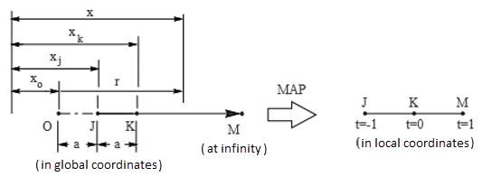
The position of the "pole," xo, is arbitrary; once chosen, the location of node K is defined by:
 | (13–395) |
The interpolation from local to global positions is performed as:
 | (13–396) |
where:

|

|
As shown,  corresponds to the global positions
  , respectively.
The global-local mapping relationship can be rewritten in terms of  , the arbitrary distance from the pole.
Solving Equation 13–396 for  yields:
 | (13–397) |
where:
 = distance from the pole O to a general point within the element = distance from the pole O to a general point within the element |
 as shown in Figure 13.40: 1-D Infinite Element Mapping as shown in Figure 13.40: 1-D Infinite Element Mapping
|
For the structural analysis, the basic solution variable  (displacement component) can be written in the polynomial forms:
 | (13–398) |
Substituting Equation 13–397 into Equation 13–398 gives:
 | (13–399) |
where  is implied, as the variable
  is assumed to vanish at infinity.
Equation 13–399 is truncated at the quadratic ( ) term in the present implementation. The equation also shows the role of the
pole position O.
) term in the present implementation. The equation also shows the role of the
pole position O.
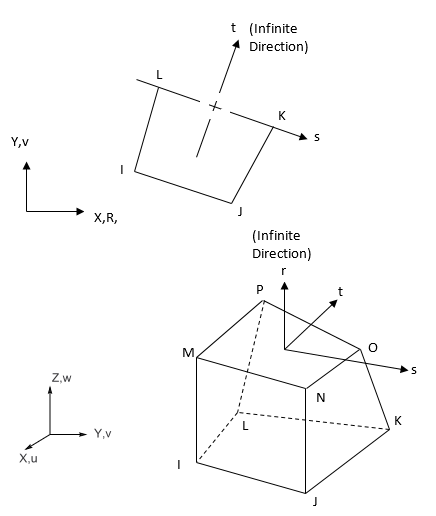
The 1-D element may be thought of as one edge of the 2-D solid infinite element, as shown:
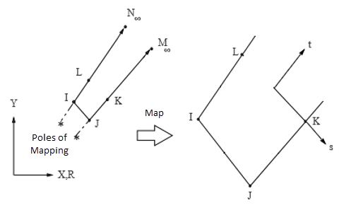
Mapping is achieved by the shape function products. The mapping functions and the
isoparametric shape functions for 2-D and axisymmetric 4 node quadrilaterals are given in 2-D and Axisymmetric 4-Node Quadrilateral Infinite Solids. The shape functions for nodes M and N are not needed as the field
variable  is assumed to vanish at infinity. 2-D mapping can be extended to 3-D in a
similarly straightforward manner.
is assumed to vanish at infinity. 2-D mapping can be extended to 3-D in a
similarly straightforward manner.
The mapping approach has an important advantage: the original Gauss-Legendre integration technique can be used with minimal modification. The only change necessary is a new calculation of the Jacobian matrix with mapping functions.
The coefficient matrix can be written as:
 | (13–400) |
where:
 = strain-displacement matrix = strain-displacement matrix |
 = elasticity matrix = elasticity matrix |
The  vectors of the
  matrix in Equation 13–164 contain the derivatives of
  with respect to the global coordinates, evaluated according to:
 | (13–401) |
where
 = Jacobian matrix which defines the geometric mapping = Jacobian matrix which defines the geometric mapping |
 is given by:
 | (13–402) |
The mapping functions  in terms of
  and
and  are given in 2-D and Axisymmetric 4-Node Quadrilateral Infinite Solids. The domain differential
  must also be written in terms of the local coordinates, so that:
 | (13–403) |
Subject to the evaluation of  and
and  , which involves the mapping functions, the element matrices
  can now be calculated in the standard manner using Gaussian quadrature.
If sudden loading occurs in an infinite elastic body, the load is not transmitted instantaneously to all parts of the body. The stresses and displacements radiate in the form of waves. The equations of equilibrium must be replaced by the equations of motion.
The equations of equilibrium without body force in an elastic medium is given by:
 | (13–404) |
where:
 = density = density |
 = particle acceleration = particle acceleration |
 = stress = stress |
 = particle position = particle position |
The stress-strain relations for an isotropic, linear elastic material can be written in
terms of Lame's constants  and
and  :
:
 | (13–405) |
where:
 = Young's modulus = Young's modulus |
 = Poisson's ratio = Poisson's ratio |
and the strain-displacement relationship is:
 | (13–406) |
By substituting Equation 13–405 and Equation 13–406 into Equation 13–404, the equations of motion can be written in terms of displacements and material properties:
 | (13–407) |
If a disturbance is produced at a point in an elastic medium, waves radiate from that point in all directions. If the medium extends to infinity, the waves can be considered as plane waves at the far field. Therefore, it may be possible to assume that all particles are moving parallel to the direction of wave propagation (dilatational wave, longitudinal wave, or p-wave), or perpendicular to that direction (distortion wave, transverse wave, or s-wave). The governing equation can be solved for the plane waves.
For the plane waves (dilatational and distortion waves), the equations of motion can be reduced in the common form:
 | (13–408) |
By comparing Equation 13–407 to Equation 13–408, we obtain:
 | (13–409) |
for the dilatational waves, and:
 | (13–410) |
for the distortion waves, where:
 = dilatational wave speed = dilatational wave speed |
 = distortion wave speed = distortion wave speed |
Any function of form  is a solution of Equation 13–408, and any function of form
  is also a solution. Therefore the general solution of the governing equation
can be represented by the form:
is also a solution. Therefore the general solution of the governing equation
can be represented by the form:
 | (13–411) |
The function  represents "forward" wave motion, and the function
  represents "backward" wave motion.
Now consider the dilatational wave that is moving forward along the x-axis. The solution is:
 | (13–412) |
The particle velocity is:
 | (13–413) |
The strain components in x-direction is:
 | (13–414) |
For the stress we have:
 | (13–415) |
The stress can be expressed in terms of wave and particle speed from Equation 13–413 through Equation 13–415:
 | (13–416) |
If we consider the backward-moving wave, the minus sign in Equation 13–416 is replaced by a plus sign.
The solution of the distortion (shear or s-) wave can be obtained in similar manner using arbitrary functions of displacements for the forward-moving waves:
 | (13–417) |
In this case, the stress component that is perpendicular to the x-direction is:
 | (13–418) |
If material discontinuity exists at  , the impinging stress wave is divided into a refracted wave and a reflected
wave. The reflected wave disturb the solution in the region
, the impinging stress wave is divided into a refracted wave and a reflected
wave. The reflected wave disturb the solution in the region  . Therefore, if the reflected wave is removed, a convex boundary can be used to
model the infinite boundary for the dynamic analysis.
. Therefore, if the reflected wave is removed, a convex boundary can be used to
model the infinite boundary for the dynamic analysis.
In typical cases, the waves are not perpendicular to the interface, so the stress components can be given in terms of normal and shear tractions:
 | (13–419) |
where:
 , ,  = normal stress and normal velocity of the particle, respectively = normal stress and normal velocity of the particle, respectively |
 , ,  = tangential stress and tangential velocity of the particle,
respectively = tangential stress and tangential velocity of the particle,
respectively |
 and and  = non-dimensional constants = non-dimensional constants |
If the constants  and
and  are set as unity, it is called the standard absorbing
boundary ([172]), and a damping matrix is built into the
structural infinite elements using the stress components in Equation 13–419.
are set as unity, it is called the standard absorbing
boundary ([172]), and a damping matrix is built into the
structural infinite elements using the stress components in Equation 13–419.