A direct finite element solution of coupled-physics problems is computationally very expensive. The goal of the reduced-order modeling is to generate a fast and accurate description of the coupled-physics systems to characterize their static or dynamic responses. The method presented here is based on a modal representation of coupled domains and can be viewed as an extension of the Mode-Superposition Method to nonlinear structural and coupled-physics systems (Gabbay, et al.([231]), Mehner, et al.([251]), Mehner, et al.([336]), and Mehner, et al.([337])).
In the mode-superposition method, the deformation state u of the structural domain is described by a factored sum of mode shapes:
 | (14–143) |
where:
| qi = modal amplitude of mode i |
| ϕi = mode shape |
| ueq = deformation in equilibrium state in the initial prestress position |
| m = number of considered modes |
By substituting Equation 14–143 into the governing equations of motion, we obtain m constitutive equations that describe nonlinear structural systems in modal coordinates qi:
 | (14–144) |
where:
| mi = modal mass |
| ξi = modal damping factor |
| ωi = angular frequency |
| WSENE = strain energy |
 = modal node force = modal node force |
 = modal element force = modal element force |
| Sl = element load scale factor (input on RMLVSCALE command) |
In a general case, Equation 14–144 are coupled since the strain energy WSENE depends on the generalized coordinates qi. For linear structural systems, Equation 14–144 reduces to Equation 14–122.
Reduced Order Modeling (ROM) substantially reduces running time since the dynamic behavior of most structures can be accurately represented by a few eigenmodes. The ROM method presented here is a three step procedure starting with a Generation Pass, followed by a Use Pass ROM144 - Reduced Order Electrostatic-Structural, which can either be performed within ANSYS or externally in system simulator environment, and finally an optional Expansion Pass to extract the full DOF set solution according to Equation 14–143.
The entire algorithm can be outlined as follows:
Determine the linear elastic modes from the modal analysis (ANTYPE,MODAL) of the structural problem.
Select the most important modes based on their contribution to the test load displacement (RMMSELECT command).
Displace the structure to various linear combinations of eigenmodes and compute energy functions for single physics domains at each deflection state (RMSMPLE command).
Fit strain energy function to polynomial functions (RMRGENERATE command).
Derive the ROM finite element equations from the polynomial representations of the energy functions.
Modes used for ROM can either be determined from the results of the test load application or based on their modal stiffness at the initial position.
Case 1: Test Load is Available (TMOD option on RMMSELECT command)
The test load drives the structure to a typical deformation state, which is representative for most load situations in the Use Pass. The mode contribution factors ai are determined from
 | (14–145) |
where:
| ϕi = mode shapes at the neutral plane nodes obtained from the results of the modal analysis (RMNEVEC command) |
| ui = displacements at the neutral plane nodes obtained from the results of the test load (TLOAD option on RMNDISP command). |
Mode contribution factors ai are necessary
to determine what modes are used and their amplitude range. Note that
only those modes are considered in Equation 14–145, which
actually act in the operating direction (specified on the RMANL command). Criterion is that the maximum of the modal
displacement in operating direction is at least 50% of the maximum
displacement amplitude. The solution vector ai indicates how much each mode contributes to the deflection state.
A specified number of modes (Nmode of the RMMSELECT command) are considered unless the mode contribution
factors are less than 0.1%.
Equation 14–145 solved by the least squares method and the results are scaled in such a way that the sum of all m mode contribution factors ai is equal to one. Modes with highest ai are suggested as basis functions.
Usually the first two modes are declared as dominant. The second mode is not dominant if either its eigenfrequency is higher than five times the frequency of the first mode, or its mode contribution factor is smaller than 10%.
The operating range of each mode is proportional to their mode
contribution factors taking into account the total deflection range
(Dmax and Dmin input on the RMMSELECT command). Modal amplitudes
smaller than 2.5% of Dmax are increased
automatically in order to prevent numerical round-off errors.
Case 2: Test Load is not Available (NMOD option on RMMSELECT command)
The first Nmode eigenmodes in the
operating direction are chosen as basis functions. Likewise, a considered
mode must have a modal displacement maximum in operating direction
of 50% with respect to the modal amplitude.
The minimum and maximum operating range of each mode is determined by:
 | (14–146) |
where:
| DMax/Min = total deflection range of the structure (input on RMMSELECT command) |
Up to 5 element loads such as acting gravity, external acceleration
or a pressure difference may be specified in the Generation Pass
and then scaled and superimposed in the Use Pass. In the same
way as mode contribution factors ai are determined
for the test load, the mode contribution factors
 for
each element load case are determined by a least squares fit:
for
each element load case are determined by a least squares fit:
 | (14–147) |
where:
 = displacements at the neutral plane nodes obtained
from the results of the element load j (ELOAD option on RMNDISP command). = displacements at the neutral plane nodes obtained
from the results of the element load j (ELOAD option on RMNDISP command). |
Here index k represents the number of modes, which have been
selected for the ROM. The coefficients
 are
used to calculate modal element forces (see Element Matrices and Load Vectors).
are
used to calculate modal element forces (see Element Matrices and Load Vectors).
In a general case, the energy functions depend on all basis functions. In the case of m modes and k data points in each mode direction one would need km sample points.
A large number of examples have shown that lower eigenmodes affect all modes strongly whereby interactions among higher eigenmodes are negligible. An explanation for this statement is that lower modes are characterized by large amplitudes, which substantially change the operating point of the system. On the other hand, the amplitudes of higher modes are reasonably small, and they do not influence the operating point.
Taking advantage of those properties is a core step in reducing the computational effort. After the mode selection procedure, the lowest modes are classified into dominant and relevant. For the dominant modes, the number of data points in the mode direction defaults to 11 and 5 respectively for the first and second dominant modes respectively. The default number of steps for relevant modes is 3. Larger (than the default above) number of steps can be specified on the RMMRANGE command.
A very important advantage of the ROM approach is that all finite element data can be extracted from a series of single domain runs. First, the structure is displaced to the linear combinations of eigenmodes by imposing displacement constrains to the neutral plane nodes. Then a static analysis is performed at each data point to determine the strain energy.
Both the sample point generation and the energy computation are controlled by the command RMSMPLE.
The objective of function fit is to represent the acquired FE data in a closed form so that the ROM FE element matrices (ROM144 - Reduced Order Electrostatic-Structural) are easily derived from the analytical representations of energy functions.
The ROM tool uses polynomials to fit the energy functions. Polynomials are very convenient since they can capture smooth functions with high accuracy, can be described by a few parameters and allow a simple computation of their local derivatives. Moreover, strain energy functions are inherent polynomials. In the case of linear systems, the strain energy can be exactly described by a polynomial of order two since the stiffness is constant. Stress-stiffened problems are captured by polynomials of order four.
The energy function fit procedure (RMRGENERATE command) calculates nc coefficients that fit a polynomial to the n values of strain energy:
 | (14–148) |
where:
| [A] = n x nc matrix of polynomial terms |
| {KPOLY} = vector of desired coefficients |
Note that the number of FE data (WSENE) points n for a mode must be larger than the polynomial order P for the corresponding mode (input on RMPORDER command). Equation 14–148 is solved by means of a least squares method since the number of FE data points n is usually much larger than the number polynomial coefficients nc.
The ROM tool uses four polynomial types (input on RMROPTIONS command):
| Lagrange |
| Pascal |
| Reduced Lagrange |
| Reduced Pascal |
Lagrange and Pascal coefficient terms that form matrix [A] in Equation 14–148 are shown in Figure 14.8: Set for Lagrange and Pascal Polynomials.
Figure 14.8: Set for Lagrange and Pascal Polynomials
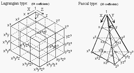
Polynomials for Order 3 for Three Modes (1-x, 2-y, 3-z)
Reduced Lagrange and Reduced Pascal polynomial types allow a further reduction of KPOLY by considering only coefficients located on the surface of the brick and pyramid respectively.
The ROM method is applicable to electrostatic-structural systems.
The constitutive equations for a coupled electrostatic-structural system in modal coordinates are:
 | (14–149) |
for the modal amplitudes and
 | (14–150) |
where:
| Ii = current in conductor i |
| Qi = charge on the ith conductor |
| Vi = ith conductor voltage |
The electrostatic co-energy is given by:
 | (14–151) |
where:
| Cij = lumped capacitance between conductors i and j (input on RMCAP command) |
| r = index of considered capacitance |
The capacitances Cij, and the electrostatic
co-energy respectively, are functions of the modal coordinates qi. As the strain energy WSENE for
the structural domain, the lumped capacitances are calculated for
each k data points in each mode direction, and then fitted to polynomials.
Following each structural analysis to determine the strain energy
WSENE, (n-1) linear simulations are performed
in the deformed electrostatic domain, where n is the number of conductors,
to calculate the lumped capacitances. The capacitance data fit is
similar to the strain energy fit described above (Function Fit Methods for Strain Energy). It is sometimes necessary to fit the inverted
capacitance function (using the Invert option
on the RMROPTIONS command).