| Matrix or Vector | Shape Functions | Integration Points |
|---|---|---|
| Stiffness Matrix | Same as attached 3-D solid or shell element | 2 x 2 or 3 x 3 |
| Load Type | Distribution |
|---|---|
| Fluid Mass Flow Rate | Fluid mass flow rate at pressure node |
| Nodal Temperature | Temperature at the pressure node |
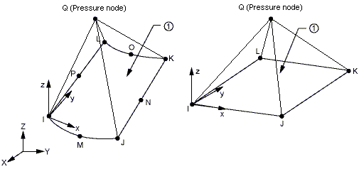
HSFLD242 is used to model fluids that are fully enclosed by solids (containing vessels). The fluid is assumed to have no viscosity, rotation or inertial effects (including acceleration loads) such as sloshing. The fluid fills the containing vessel completely so it has no free surface. Under these conditions, the fluid can be assumed to be hydrostatic; that is, the fluid pressure is uniform throughout the fluid volume. The hydrostatic fluid element is pyramid shaped with the base overlaying a 3-D solid or shell element face and the vertex at a pressure node. The element nodes shared with the underlying 3-D solid or shell element have only translation degrees of freedom. The pressure node has a single hydrostatic pressure degree of freedom (HDSP) and is shared by all hydrostatic fluid elements defining the fluid volume. The coupling between the fluid volume and the containing vessel is modeled by applying the hydrostatic fluid pressure as a surface load on the containing vessel. No fluid is assumed to flow in or out of the containing vessel unless a hydrostatic pressure value or fluid mass flow rate is prescribed at the pressure node.
Formulating a coupled system of a solid (containing vessel) enclosing a hydrostatic fluid requires augmenting the internal virtual work for the solid with contributions from the fluid. Starting with the rate of internal energy expression:
 | (13–368) |
where:
| W = internal energy for the solid |
| Ss = current solid surface enclosing the fluid volume |
| Sf = current fluid surface enclosing the fluid volume |
| tsi = component i of surface traction at a point on Ss |
| tfi = component i of surface traction at a point on Sf |
| vsi = component i of velocity at a point on Ss |
| vfi = component i of velocity at a point on Sf |
Since the fluid fills the containing vessel completely and the system is in equilibrium, the surface traction at a point on the solid surface should be equal and opposite to the surface traction at a point on the fluid surface that it is in contact with. The surface tractions represent the loads exerted by the fluid and the solid on each other. Assuming no viscosity for the fluid, the surface tractions have only normal non-zero components, so:
 | (13–369) |
where:
| P = fluid pressure |
| ni = component i of outward normal to the fluid surface enclosing the fluid volume |
Further, assuming that the fluid has no inertial effects or acceleration loads, Equation 8–2 for fluid momentum show that the fluid pressure should be uniform. Using this fact with Equation 13–369 in Equation 13–368 gives:
 | (13–370) |
By taking a variation of Equation 13–370 and then using Gauss' theorem, we get the internal virtual work expression:
 | (13–371) |
where:
| Vf = current fluid volume |
| vfi,i = div v f = divergence of velocity vector at a point in Vf |
The second term on the right hand side in Equation 13–371 is the virtual work done by the hydrostatic fluid pressure on the solid that contains the fluid and represents the coupling between the fluid volume and the solid (containing vessel).
Since the fluid volume has uniform pressure, the volumetric strain is also uniform. This allows Equation 13–371 to be simplified further.
Using the definitions of deformation gradient and its determinant as given in Equation 3–2, Equation 3–3, and Equation 3–4, and the derivative of the determinant (Gurtin [382]), it can be seen that:
 | (13–372) |
Similarly, for the solid surface enclosing the fluid volume:
 | (13–373) |
where:
| Vs = current volume enclosed by solid surface Ss |
Using Equation 13–372 and Equation 13–373 (and its variation) in Equation 13–371 gives:
 | (13–374) |
The internal virtual work in Equation 13–374 is valid for large as well as small strains. Since the fluid is assumed to have no acceleration loads or free surface, there are no contributions to external virtual work from loads. However, if fluid mass flow rate is prescribed at the pressure node, then the mass, and hence the volume, of the fluid will change and the virtual work expression will be:
 | (13–375) |
where:
| w = fluid mass flow rate (use F command) |
| ρf = current fluid density |
The stiffness matrix for the coupled system can be obtained by taking the derivative of the virtual work expression as given in Equation 13–375:
 | (13–376) |
For completeness, the variational quantities in Equation 13–376 need to be
expressed in terms of the independent variables. To compute  , we start by taking a variation of Equation 13–373:
 | (13–377) |
Since the fluid is assumed to be irrotational, there is no contribution from the term containing the variation of the normal, δni.
For  , we start with Equation 13–377, including the term
containing the variation of the normal:
, we start with Equation 13–377, including the term
containing the variation of the normal:
 | (13–378) |
Again, irrotational fluid assumption eliminates terms with variation of the normal. If t 1 and t 2 define orthonormal tangent vectors on the surface such that:
 | (13–379) |
then, Equation 13–378 can be expanded as:
 | (13–380) |
The terms  and Dρf in Equation 13–376
define material stiffness for the fluid volume. This requires the definition of the
pressure-volume relationship as described below.
and Dρf in Equation 13–376
define material stiffness for the fluid volume. This requires the definition of the
pressure-volume relationship as described below.
The incompressibility constraint for the fluid volume can be given by using Equation 13–372 as:
 | (13–381) |
The augmented virtual work expression incorporating the incompressibility constraint can be written as:
 | (13–382) |
where:
| λ = Lagrange multiplier |
Comparing Equation 13–382 to Equation 13–375 shows that they are equivalent with the hydrostatic fluid pressure P acting as a Lagrange multiplier. The stiffness contribution can be obtained by taking the derivative of the augmented virtual work:
 | (13–383) |
The incompressible fluid may have a change in volume if it has non-zero thermal expansion. Since temperature is not defined as a degree of freedom, changes in volume due to temperature changes are computed by specifying temperature loading (use the BF command) and coefficient of thermal expansion (use the MP command):
 | (13–384) |
where:
| α = coefficient of thermal expansion (use MP command) |
 = rate of change of temperature = rate of change of temperature |
| V0f = initial fluid volume |
When KEYOPT(6) = 1, the change in volume is accommodated by a change in fluid mass (mass flows into or out of the cavity). When KEYOPT(6) = 2, the change in volume is accommodated by a change in fluid density such that the fluid mass is held constant.
Using the constitutive equation for liquid (see Fluid Material Models), the rate of change of volume and its variation can be given as:
 | (13–385) |
 | (13–386) |
where:
K = bulk modulus (use TB command with Lab = FLUID and TBOPT =
LIQUID) |
The variation of current density can be defined as:
 | (13–387) |
To define the rate of change of volume, we need to look at incremental change in volume:
 | (13–388) |
where:
| Δt = time increment for current substep |
| Vnf = fluid volume at the end of previous substep |
Using the Ideal Gas Law, the previous expression can be expanded as:
 | (13–389) |
where:
| Pt = Pref + P = total fluid pressure |
| Pref = reference pressure (specified as a real constant with R command) |
| Tt = Toff + T = total temperature |
| Toff = temperature offset from absolute zero to zero (use TOFFST command) |
| Pnt = total fluid pressure at the end of previous substep |
| Tnt = total temperature at the end of previous substep |
The variation of the rate of change of volume can be easily obtained as:
 | (13–390) |
and the variation of current density can be given as:
 | (13–391) |
For compressible fluids that do not follow the constitutive equation for liquid or the Ideal Gas Law, the rate of change of volume can be expressed as:
 | (13–392) |
where:
 = slope (interpolated) of the pressure-volume data
curve = slope (interpolated) of the pressure-volume data
curve |
 = slope (interpolated) of the temperature-volume data
curve = slope (interpolated) of the temperature-volume data
curve |
and the variation of the rate of change of volume can be expressed as:
 | (13–393) |
The variation of current density is defined as:
 | (13–394) |
See Fluid Material Models for more details.