Continuum stress elements represent the volume of a model used for deflection and stress analysis. They do not include shell, surface, contact, beam, pipe or other special elements.
Continuum stress elements have few, if any, basic deformation assumptions and are the primary elements for stress analysis, especially for solid structures.
Elements can be either 2-D or 3-D and are usually obtained by meshing areas or volumes. They can be used for any structural analysis.
Although continuum stress elements may not be computationally efficient for structures having one or two dimensions that are much smaller than the remaining dimension(s), they are still useful for benchmarking purposes, or to obtain more detailed results for such structures.
The following topics related to continuum elements are available:
The following topics about stress states in continuum elements assumes global Cartesian directions and applies to the PLANE182 and PLANE183 elements unless otherwise noted:
Plane stress is a stress state that varies only in the X and Y directions. The stress in the Z direction is always zero, as are the XZ and YZ shear stresses.
Plane stress is generally used on flat, thin structures, where the deformation is assumed to be solely in the plane of the structure. For example, flat plates pulled in tension may be analyzed with plane stress. Although a unit thickness is generally assumed, you can input a thickness as well.
Plane strain is a stress state that varies only in the X and Y directions. The strain in the Z direction is always zero, as are the XZ and YZ shear strains.
Plane strain is generally used on thick structures such as the cross-section of a dam.
Generalized plane strain is similar to plane strain, except that the Z direction strain is not required to be zero. The Z direction strain may vary linearly in the X and Y directions (but not in the Z direction), removing the implied restriction of plane strain that the model extends without limit in the Z direction. The model in the Z direction can also have a uniform curvature.
Generalized plane strain can be used for modeling a section of cylindrical geometries, or to model long structures with a load at the end.
For more information, see Generalized Plane Strain Options.
Axisymmetric geometry is defined in the X-Y plane with positive X values. The geometry can be thought of as the cross-section, which, when rotated about the global Cartesian Y axis, forms the actual model. Unless otherwise described, therefore, the model and the loading and deformations are constant around the circumference.
An axisymmetric analysis can be used for a nuclear containment building under internal pressure or vertical earthquake.
Axisymmetric geometry is defined in the X-Y plane with positive X values. The geometry can be thought of as the cross-section, which, when rotated about the global Cartesian Y axis, forms the actual model. Unless otherwise described, therefore, the model and the loading and deformations are constant around the circumference. Axisymmetric deformation can include the torsion about the global Cartesian Y axis.
An axisymmetric analysis can be used for a nuclear containment building under internal pressure or vertical earthquake.
Besides PLANE182 and PLANE183, SHELL208 and SHELL209 support axisymmetric analyses.
General axisymmetric is the same as axisymmetric except that the deformations can be nonaxisymmetric.
ANSYS, Inc. recommends using the SOLID272 and SOLID273 elements to simulate general axisymmetric characteristics. The general axisymmetric elements offer the following benefits:
The deformations can be nonaxisymmetric.
The deformations are modeled internally as a Fourier series, with all terms of the Fourier series solved simultaneously.
All nonlinearities are supported.
An example general axisymmetric application is simulating threaded pipe connections.
For more information, see General Axisymmetric Elements.
Alternatively, general axisymmetric can be simulated with harmonic axisymmetric elements when the problem is linear.
The deformations are modeled as a Fourier series, with each term of the Fourier series solved separately and then combined in postprocessing, and you must perform both tasks manually. Supported elements are PLANE25, PLANE83, and SHELL61.
Only linear behavior is supported.
An example axisymmetric-harmonic application is simulating a nuclear containment building subjected to a horizontal earthquake.
For more information, see Harmonic Axisymmetric Elements.
|
Due to the limitations of axisymmetric-harmonic elements, ANSYS, Inc. recommends using general axisymmetric elements instead. The method presented here is provided for legacy support only. |
Traditional isoparametric continuum elements have never been sufficiently robust or accurate enough for general stress analysis.
Even in a linear analysis, lower-order elements are prone to shear locking in bending-dominated problems. Both lower- and higher-order elements experience volumetric locking when materials are incompressible or nearly incompressible, yet most nonlinear materials are either nearly or fully incompressible.
Current-technology continuum elements are available to overcome such problems. As technology advances, ANSYS, Inc. continues to develop robust new element types using the latest technologies available. Current-technology elements are more advanced and feature-rich than legacy elements.
The following topics concerning current element technologies for general stress analysis are available:
The following current technologies are available for lower-order quad and brick elements:
The B-bar (  ) method helps to prevent volumetric locking in nearly
incompressible cases. It replaces volumetric strain at the Gauss integration
point with the average volumetric strain of the elements.
) method helps to prevent volumetric locking in nearly
incompressible cases. It replaces volumetric strain at the Gauss integration
point with the average volumetric strain of the elements.
This method cannot, however, prevent any shear locking in bending-dominated problems. In such cases, use the enhanced strain formulation of the element. If it is not clear whether the deformation is bending-dominated, the enhanced strain formulation is still recommended.
This technology can be used with mixed u-P formulations.
The enhanced strain formulation prevents shear locking in bending-dominated problems and volumetric locking in nearly incompressible cases. The formulation introduces certain number of internal (and inaccessible) degrees of freedom to overcome shear locking, and an additional internal degree of freedom for volumetric locking (except for the case of plane stress in 2-D elements). All internal degrees of freedom are introduced automatically at the element level and condensed out during the solution phase of the analysis.
Because of the extra internal degrees of freedom and static condensation,
the enhanced strain formulation option is less efficient than either the
 method (selective reduced integration)
option or the uniform reduced
integration option.
method (selective reduced integration)
option or the uniform reduced
integration option.
This technology can be used with mixed u-P formulations.
The simplified enhanced strain formulation prevents shear locking in bending-dominated problems. This formulation is similar to the enhanced strain formulation, except that it introduces only the internal degrees of freedom necessary to prevent shear locking. For the plane stress state, this formulation is identical to the enhanced strain formulation.
Because there are no internal degrees of freedom to handle volumetric locking, this formulation is not ideal when the material is nearly incompressible, except when also using the mixed u-P formulation. When used with mixed u-P, the simplified enhanced strain formulation yields the same results as the enhanced strain formulation. All internal degrees of freedom are introduced automatically at the element level and condensed out during the solution phase of the analysis.
The uniform reduced integration method helps to prevent shearing locking
in bending-dominated problems and volumetric locking in nearly
incompressible cases. Because it has only one integration point, this option
is more efficient than the  method (selective reduced integration)
and the enhanced strain
formulations. Because the artificial energy introduced to control the
hourglass effect can diminish solution accuracy, however, consider this
option last.
method (selective reduced integration)
and the enhanced strain
formulations. Because the artificial energy introduced to control the
hourglass effect can diminish solution accuracy, however, consider this
option last.
When using uniform reduced integration, verify the solution accuracy by comparing the total energy (SENE label on the ETABLE command) and the artificial energy (AENE label on the ETABLE) introduced by hourglass control. If the ratio of artificial energy to total energy is less than five percent, the solution is generally acceptable. If the ratio exceeds five percent, refine the mesh. You can also monitor the total energy and artificial energy during the solution phase of the analysis (OUTPR,VENG).
Linear tetrahedron elements use mixed u-P formulation with pressure stabilization. The program achieves stabilization by enhancing the strain field with three internal degrees of freedom (which are condensed out at the element level). The stabilization allows for a robust and accurate element.
Higher-order elements (actually second-order here) do not have shear locking due to the quadratic shape functions, but they are prone to volumetric locking if the full-integration scheme is used. To avoid this problem, higher-order elements use uniform reduced integration as the default or only option.
The hourglass effect is not an issue if the model has at least two elements for 2-D problems, or at least two elements in each direction for 3-D problems, as it is difficult for hourglass mode to propagate beyond one element. Hourglass control is therefore not needed.
Uniform reduced integration can be used with mixed u-P formulation.
The full integration option is used primarily for linear analysis, and for nonlinear analysis, uniform reduced integration is the better choice. If full integration is necessary for an analysis involving nonlinear material, use it with mixed u-P formulation to limit the risk of volumetric locking.
The second-order elements do not have shear locking, and volumetric locking is generally not an issue. If you observe volumetric locking, used mixed u-P formulation.
Mixed u-P elements use both displacement and hydrostatic pressure as primary unknown variables. Mixed u-P formulation is available in SOLID285, and in most other current-technology elements where KEYOPT(6) > 0, such as: PLANE182, PLANE183, SOLID185, SOLID186, SOLID187, SOLSH190, SOLID272, and SOLID273.
The following related topics are available:
Incompressible material behavior may lead to difficulties in numerical simulation, such as volumetric locking, inaccuracy of solution, checkerboard pattern of stress distributions, or, occasionally, divergence. Mixed u-P elements are intended to overcome these problems.
Lagrange multiplier based mixed u-P elements (current-technology solid elements with KEYOPT(6) > 0 and SOLID285) can also be used to overcome incompressible material problems. They are designed to model material behavior with high incompressibility such as fully or nearly incompressible hyperelastic materials and nearly incompressible elastoplastic materials (high Poisson ratio or undergoing large plastic strain). Lagrange multipliers extend the internal virtual work so that the volume constraint equation is included explicitly. This introduces hydrostatic pressure (or volume change rate for nearly incompressible hyperelastic materials) as a new independent variable. Unlike the hyperelastic elements, the hydrostatic pressure variables are not condensed on the element level, but are solved at the global level. For more infomration, see u-P Formulation II in the Mechanical APDL Theory Reference.
The mixed u-P formulation of the current-technology solid elements offers options for handling
incompressible material behavior. You can combine the mixed u-P formulation with
other element technologies such as the  method (also known as the selective reduced integration
method) and the uniform reduced integration method. With current-technology
elements, you can combine the mixed u-P formulation with the enhanced strain
formulation method. Furthermore, the mixed u-P formulation is associated with
hyperelastic models, such as Mooney-Rivlin, Neo-Hookean, Ogden, Arruda-Boyce,
polynomial form, and user-defined.
method (also known as the selective reduced integration
method) and the uniform reduced integration method. With current-technology
elements, you can combine the mixed u-P formulation with the enhanced strain
formulation method. Furthermore, the mixed u-P formulation is associated with
hyperelastic models, such as Mooney-Rivlin, Neo-Hookean, Ogden, Arruda-Boyce,
polynomial form, and user-defined.
The number of independent hydrostatic pressure degrees of freedom depends on the element type, element technology, and the value of KEYOPT(6), as shown in Table 5.1: Number of Independent Pressure Degrees of Freedom in One Element.
Table 5.1: Number of Independent Pressure Degrees of Freedom in One Element
| Element | Basic Element Technology | KEYOPT(6) | Number of Pressure DOFs | Interpolation Function |
|---|---|---|---|---|
| PLANE182 |
 method (selective reduced integration)
or uniform reduced
integration method (selective reduced integration)
or uniform reduced
integration | 1 | 1 | Constant |
| PLANE182 | Enhanced strain formulation | 1 | 3 | Linear |
| PLANE183 | Uniform reduced integration (KEYOPT(1) = 0) | 1 | 3 | Linear |
| PLANE183 | 3-point integration (KEYOPT(1) = 1) | 1 | 3 | Linear |
| SOLID185 |
 method (selective reduced integration)
or uniform reduced
integration method (selective reduced integration)
or uniform reduced
integration | 1 | 1 | Constant |
| SOLID185 | Enhanced strain formulation | 1 | 4 | Linear |
| SOLID186 | Uniform reduced integration | 1 | 4 | Linear |
| SOLID186 | Full integration | 1 | 4 | Linear |
| SOLID187 | 4-point integration | 1 | 1 | Constant |
| SOLID187 | 4-point integration | 2 | 4 | Linear |
| SOLSH190 | Enhanced strain formulation | 1 | 4 | Linear |
| SOLID272 | Full integration in the r-z plane. | 1 | KEYOPT(2) | Constant in the r-z plane and Fourier interpolation in the circumferential (θ) direction |
| SOLID273 | Uniform integration in the r-z plane. | 1 | KEYOPT(2) x 3 | Linear in the r-z plane and Fourier interpolation in the circumferential (θ) direction |
| SOLID285 | Stabilized pressure formulation | --- | 4 | Linear |
The hydrostatic pressure has an interpolation function one order lower than the one for volumetric strain. Therefore, elastic strain only agrees with stress in an element on the average instead of point-wise.
For current-technology mixed u-P elements, the volume constraint equation is checked for each element of a nonlinear analysis. The number of elements in which the constraint equation is not satisfied is reported in the output file. The default tolerance for the volumetric compatibility or volume constraint check is 1.0 x 10⁻³. You can change this value if necessary (CNVTOL).
For the SOLID285 element, hydrostatic pressure is added as a degree of freedom at each node. The incompressibility is therefore checked at each node (similar to forces). For more information, see the documentation for the CNVTOL command.
The mixed u-P formulation is not needed in plane stress; the incompressibility condition is assumed, and the thickness is adjusted based on this incompressible assumption. For 2-D elements PLANE182 and PLANE183, using the mixed u-P formulation with either of the plane stress options (KEYOPT(3) = 0 or 3), the program resets any KEYOPT(6) setting to 0 automatically for pure displacement formulation.
Incompressible material behavior can be divided into two categories: fully incompressible materials and nearly incompressible materials. Typical fully incompressible materials are hyperelastic materials. You must use a current-technology element with mixed u-P formulation or SOLID285 to model this material behavior. For element SOLID187, set KEYOPT(6) = 1.
Nearly incompressible materials include hyperelastic materials and elastoplastic materials. The current-technology elements with mixed u-P formulation and SOLID285 are available for nearly incompressible hyperelastic materials.
The best element choice varies from problem to problem, as indicated in these general guidelines:
For material behavior with very small compressibility: Use a current-technology element with mixed u-P formulation or SOLID285.
For moderate compressibility: Use PLANE182/SOLID185 with
 (most efficient), a current-technology element with mixed u-P formulation,
or SOLID285.
(most efficient), a current-technology element with mixed u-P formulation,
or SOLID285. When deformation is highly confined: Use a current-technology element with mixed u-P formulation.
Nearly incompressible elastoplastic materials are materials with Poisson's ratio close to 0.5, or elastoplastic materials undergoing very large plastic deformation. For such cases, especially when the deformation is close to being fully incompressible, the mixed u-P formulation of the current-technology elements and SOLID285 is more robust, yielding better performance. Try pure displacement formulation (KEYOPT(6) = 0) first, however, because the extra pressure degrees of freedom are involved in mixed formulation. If you are using mixed formulation with element SOLID187, it is good practice to specify hydrostatic pressure interpolation (KEYOPT(6) = 2).
Avoid overconstrained models when using current-technology elements with mixed u-P formulation. An
overconstrained model means that globally or locally, the number of displacement
degrees of freedom without any prescribed values (Nd)
is less than the number of hydrostatic pressure degrees of freedom
(Np). Np can be
calculated by the number of elements times the number of pressure degrees of
freedom within each element. (See Table 5.1: Number of Independent Pressure Degrees of Freedom in One Element for the
specific numbers used with the current-technology elements.) If different type
elements are included, Np is the summation of the
products over each type of mixed formulation element. The overconstrained
problem can be overcome by increasing the number of nodes without any
displacement boundary conditions, or by refining the mesh. The optimal values
for Np and Nd are
Nd/Np = 2 for 2-D problems and
Nd/Np = 3 for 3-D problems.
On the other hand, SOLID285 is not likely to be
overconstrained. At each node, it has one pressure degree of freedom and three
degrees of freedom (UX, UY, and UZ). These are the best values for
Nd/Np.
When the mixed u-P formulation of the current-technology plane and solid elements is applied to fully incompressible hyperelastic materials, you must also avoid the “no unique solution” situation. No unique solution occurs if all boundary nodes have prescribed displacements in each direction and the material is fully incompressible. Since hydrostatic pressure is independent from deformation, it should be determined by the force/pressure boundary condition. If no force/pressure boundary condition is applied, the hydrostatic pressure cannot be determined, or the solution is not unique. In this case, any stress field in equilibrium would be still in equilibrium and not cause any further deformation by adding an arbitrary value of hydrostatic pressure. This problem can be solved simply by having at least one node on the boundary in at least one direction without a prescribed displacement boundary condition. This direction cannot be the tangential direction of the boundary at this node. That means the solution is the particular one with zero force at the node in that direction where no displacement is prescribed.
The generalized plane strain feature assumes a finite deformation domain length in the Z direction, rather than the infinite value assumed for standard plane strain. Generalized plane strain, therefore, gives more practical results for deformation problems where the Z-direction dimension is not long enough. It also offers a more efficient way to simulate certain 3-D deformations using 2-D element options.
The deformation domain or structure is formed by extruding a plane area along a curve with a constant curvature, as shown in the following figure:

The extrusion begins at the starting (or reference) plane and stops at the ending plane. The curve direction along the extrusion path is called the fiber direction. The starting and ending planes must be perpendicular to this fiber direction at the beginning and ending intersections.
If the boundary conditions and loads in the fiber direction do not change over the course of the curve, and if the starting plane and ending plane remain perpendicular to the fiber direction during deformation, then the amount of deformation of all cross sections is identical throughout the curve, and does not vary at any curve position in the fiber direction. Any deformation, therefore, can be represented by the deformation on the starting plane, and the 3-D deformation can be simulated by solving the deformation problem on the starting plane. The existing plane strain and axisymmetric options are particular cases of the generalized plane strain option.
All inputs and outputs are in the global Cartesian coordinate system. The starting plane must be the X-Y plane, and must be meshed. The applied nodal force on the starting plane is the total force along the fiber length. The geometry in the fiber direction is specified by the rotation about X and Y of the ending plane and the fiber length passing through a point that you specify on the starting plane, called the starting (or reference) point. The starting point creates an ending point on the ending plane through the extrusion process. The boundary conditions and loads in the fiber direction are specified by applying displacements or forces at the ending point. This ending point can be different from regular nodes, in that it is designated by the same X-Y coordinates that are fixed in plane during deformation.
The generalized plane strain option introduces three new degrees of freedom for each element. Two internal nodes are created automatically at the solution stage for the generalized plane strain option to carry the extra three degrees of freedom. You can apply boundary conditions and loads and check the results of the fiber length and rotation angle changes, and reaction forces, using the commands GSBDATA, GSGDATA, GSSOL, and GSLIST. The results of the fiber length change, rotation angle change, and reaction forces can also be viewed through OUTPR.
The fiber length change is positive when the fiber length increases. The sign of the rotation angle or angle change is determined by how the fiber length changes when the coordinates of the ending point change. If the fiber length decreases when the X coordinate of the ending point increases, the rotation angle about Y is positive. If the fiber length increases when the Y coordinate of the ending point increases, the rotation angle about X is positive.
In Eigenvalue analyses, such as Eigen buckling and modal analysis, the generalized plane strain option usually reports fewer Eigenvalues and Eigenvectors than you would obtain in a 3-D analysis. Because it reports only homogeneous deformation in the fiber direction, generalized plane strain employs only three degrees of freedom to account for these deformations. The same 3-D analysis would incorporate many more degrees of freedom in the fiber direction.
Because the mass matrix terms relating to degrees of freedom in the fiber direction are approximated for modal and transient analyses, you cannot use the lumped mass matrix for these types of analyses, and the solution may be slightly different from regular 3-D simulations when any of the three designated degrees of freedom is not restrained.
Axisymmetric problems should be modeled using axisymmetric elements. An axisymmetric model greatly reduces the modeling and analysis time compared to that of an equivalent 3-D model.
If loading is also axisymmetric, the analysis is relatively straightforward. However, loading often varies around the circumference. Two methods are available for handling nonaxisymmetric loading:
General Axisymmetric Elements -- Support any type of material or loading
Harmonic Axisymmetric Elements -- Restricted to linear materials and sinusoidal loading.
Different from harmonic axisymmetric elements, general axisymmetric elements (SOLID272, SOLID273, and SURF159) introduce the Fourier series into the interpolation functions to describe the change of displacements in the circumferential (θ) direction. The elements can therefore apply to any analysis type, including geometric nonlinear analyses, and can support any load and deformation mode. For more information, see SOLID272 - General Axisymmetric Solid with 4 Base Nodes and SOLID273 - General Axisymmetric Solid with 8 Base Nodes in the Mechanical APDL Theory Reference.
The elements can have any axis as the axisymmetric axis (defined via SECTYPE and SECDATA commands). You need only define base elements on a flat plane.
The NAXIS command automatically creates a full 3-D finite-element model using the base elements, the axisymmetric axis, and the number of Fourier nodes specified via KEYOPT(2). The axisymmetric axis must be on the master plane, and the base elements must be on one side of the axis. A base element or base node must be associated with one axisymmetric axis before issuing the NAXIS command. All generated nodes are equally distributed circumferentially.
The default element coordinate system is a cylindrical coordinate system having the axisymmetric axis as z, the origin defined via the SECDATA command, and θ = 0 at the master plane. The right-hand rule determines the direction of θ, resulting in x(r), y(θ), and z from the right-hand coordinate system, as shown:
The displacements in the r, θ, and z directions, however, are interpolated by
ui = hi(s,t)(c1 + a1cosθ + b1sinθ + a2cos2θ + b2sin2θ + a3cos3θ + b3sin3θ . . .)
where
i = r, θ, z
and
hi(s,t) is the standard interpolation function for 2-D elements.
The nodes can have their own coordinate systems defined in any direction, as is the case with the nodes of any other solid element. For more detailed information, see General Axisymmetric Solids in the Mechanical APDL Theory Reference.
General axisymmetric elements differ from harmonic axisymmetric elements in that you do not specify the symmetric and unsymmetric terms, input peak values of loads, and solve for each term as one load step. Instead, you apply all physical loads (forces and displacements) at the nodes and solve the problem only once to obtain the solution.
The order of hi(s,t) is determined by the element type. (SOLID272 is a lower-order element and SOLID273 is a higher-order element.) The order of Fourier terms is determined by the number of Fourier nodes, or the number of nodes created in the circumferential direction for one base node (including the base node itself). This number is also the number of nodal planes in the circumferential direction, which you input via the element's KEYOPT(2). The KEYOPT(2) setting, the number of Fourier nodes, and the Fourier terms are shown in Table 5.2: Fourier Terms for General Axisymmetric Elements. Generally, each Fourier term has different coefficients except when KEYOPT(2) is an even number (in which case the highest terms of the sine and cosine have the same coefficient).
Table 5.2: Fourier Terms for General Axisymmetric Elements
| KEYOPT(2) Value | Number of Fourier Nodes (and Nodal Planes) | Fourier Terms | Degrees Between Nodal Planes |
|---|---|---|---|
| 1 | 1 | c1 | 360 |
| 3 | 3 | c1, a1cosθ, b1sinθ | 120 |
| 4 | 4 | c1, a1cosθ, b1sinθ, a2cos2θ, a2sin2θ | 90 |
| 5 | 5 | c1, a1cosθ, b1sinθ, a2cos2θ, b2sin2θ | 72 |
| 6 | 6 |
c1, a1cosθ, b1sinθ, a2cos2θ, b2sin2θ, a3cos3θ, a3sin3θ | 60 |
| 7 | 7 |
c1, a1cosθ, b1sinθ, a2cos2θ, b2sin2θ, a3cos3θ, b3sin3θ | 51.43 |
| 8 | 8 |
c1, a1cosθ, b1sinθ, ... , a4cos4θ, a4sin4θ | 45 |
| 9 | 9 |
c1, a1cosθ, b1sinθ, ... , a4cos4θ, b4sin4θ | 40 |
| 10 | 10 |
c1, a1cosθ, b1sinθ, ... , a5cos5θ, a5sin5θ | 36 |
| 11 | 11 |
c1, a1cosθ, b1sinθ, ... , a5cos5θ, b5sin5θ | 32.73 |
| 12 | 12 |
c1, a1cosθ, b1sinθ, ... , a6cos6θ, a6sin6θ | 30 |
For KEYOPT(2) = 1, the deformation is also axisymmetric but, unlike the axisymmetric option of 2-D elements such as PLANE182, the general axisymmetric elements allow torsion. If no torsion load exists, it is more efficient to use the axisymmetric elements.
To simulate unsymmetric deformation, set KEYOPT(2) > 1. The greater the number of Fourier nodes, the more accurate the simulation of complicated deformation modes.
Solve localized deformation problems with a greater number of Fourier nodes (higher-order Fourier terms). Be aware that the deformation is not as localized as it would be when using standard 3-D solid elements; with general axisymmetric elements, displacements are interpolated using Fourier terms in the circumferential direction (rather than being interpolated piecewise using linear/quadratic functions as in 3-D solid elements).
Contact is usually a local phenomenon. Generally, higher-order Fourier terms are necessary.
The maximum allowed number of Fourier nodes is 12. If more than 12 nodes are necessary, a general axisymmetric element may not be computationally efficient; therefore, it is better to use a standard 3-D solid element for such cases.
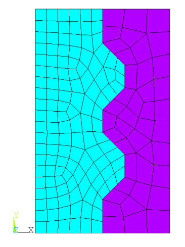
The following example input file shows how to use commands and the SOLID272 element to generate a 3-D general axisymmetric model. The model represents a simple thread connection made of two parts, a bolt and a nut, both modeled with 12 Fourier nodes (KEYOPT(2) = 12) and the global Y axis as the axis of symmetry.
/batch,list
/title, Sample input for generating general axisymmetric solid elements
/prep7
!
et,1,272,,12       !define general axisymmetric SOLID272 with 12 nodes along circumferential direction
et,2,272,,12
!
sect,1,axis        !define general axisymmetric section
secd,2,0,2         !use pattern 2 with global cartesian coordinate system (0)and y as axis of symmetry (2)
!
mp,ex,1,2.0e5      !define elastic material properties
mp,nuxy,1,0.3
!
!
! Create  2D  geometry of thread connection (bolt/nut)
!
k,1,1.0,0
k,2,4.0,0
k,3,4,1.5
k,4,5.0,2.5
k,5,5.0,3.5
k,6,4.0,4.5
k,7,4.0,5.5
k,8,5.0,6.5
k,9,5.0,7.5
k,10,4.0,8.5
k,11,4.0,10
k,12,1.0,10
k,13,7.0,0
k,14,7.0,10
!
k,15,4.0,0
k,16,4,1.5
k,17,5.0,2.5
k,18,5.0,3.5
k,19,4.0,4.5
k,20,4.0,5.5
k,21,5.0,6.5
k,22,5.0,7.5
k,23,4.0,8.5
k,24,4.0,10
!
a,1,2,3,4,5,6,7,8,9,10,11,12
a,15,16,17,18,19,20,21,22,23,24,14,13
!
!
!Mesh 2D geometry
!
esize,0.5
type,1             !use type 1 for bolt component
mat,1
secn,1             !use general axisymmetric section
amesh,1            !generate the master plane nodes and elements for bolt component
!
esize,1            !use different mesh
type,2             !use type 2 for nut component
mat,1
secn,1             !use general axisymmetric section
amesh,2            !generate the master plane nodes and elements for nut component
!
/PNUM,TYPE,1       !display element type numbers
/NUMBER,1          !numbering shown with colors only
eplot              !visualise the 2D model
!
!
!Generate full 3D axisymmetric model of bolt and nut using 12 planes
!
naxis
!
/view,1,1,1,1      !isometric view
!
nplot              !display the 12 nodal planes along circumferential direction
!
/eshape,1          !display elements with general axisymmetric shape
!
esel,s,type,,1     !display 3D axisymmetric model of bolt
eplot
!
esel,s,type,,2     !display 3D axisymmetric model of nut
eplot
!
esel,all
!
eplot              !display full 3D axisymmetric model of bolt and nut
!
fini
The input listing generates the following 2-D and 3-D meshes:
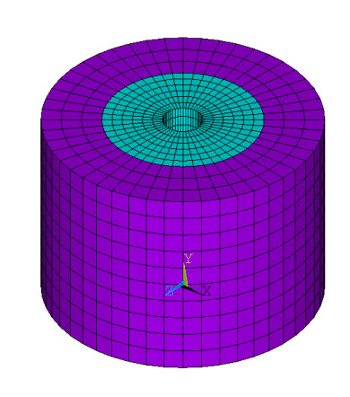
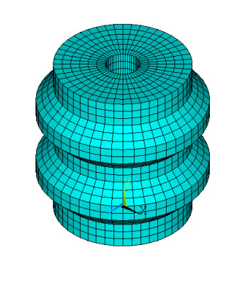
The general axisymmetric elements representing the bolt and nut are shown separately in the figures below:
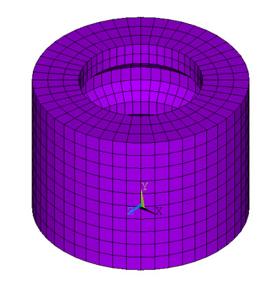
An axisymmetric structure can be represented by a plane (X,Y) finite-element model.
ANSYS, Inc. recommends general axisymmetric elements SOLID272 and SOLID273 for such applications because they can accept any type of load and can support nonlinear analyses. However, you can also use a special class of axisymmetric elements called harmonic elements: PLANE25, SHELL61, PLANE75, PLANE78, and PLANE83. The harmonic elements allow a nonaxisymmetric load and support linear analyses.
Axisymmetric elements are modeled on a 360° basis, so all input and output nodal heat flows, forces, moments, fluid flows, current flows, electric charges, magnetic fluxes, and magnetic current segments must be input in this manner. Similarly, input real constants representing volumes, convection areas, thermal capacitances, heat generations, spring constants, and damping coefficients must also be input in on a 360° basis.
Unless otherwise stated, the model must be defined in the Z = 0.0 plane. The global Cartesian Y axis is assumed to be the axis of symmetry. Further, the model is developed only in the +X quadrants. Hence, the radial direction is in the +X direction.
The boundary conditions are described in terms of the structural elements. The forces (FX, FY, etc.) and displacements (UX, UY, etc.) for the structural elements are input and output in the nodal coordinate system. All nodes along the y axis centerline (at x = 0.0) should have the radial displacements (UX if not rotated) specified as zero, unless a pinhole effect is desired. At least one value of UY should be specified or constrained to prevent rigid body motions. Torsion, while axisymmetric, is available only for a few element types. If an element type allows torsion, all UZ degrees of freedom should be set to 0.0 on the centerline, and one node with a positive X coordinate must also have a specified or constrained value of UZ. Pressures and temperatures may be applied directly. Acceleration, if any, is usually input only in the axial (Y) direction. Similarly, angular velocity, if any, is usually input only about the Y axis.
For more information, see Harmonic Axisymmetric Elements with Nonaxisymmetric Loads.
An axisymmetric structure (defined with the axial direction along the global Y axis and the radial direction parallel to the global X axis) can be represented by a plane (X, Y) finite-element model. The use of an axisymmetric model greatly reduces the modeling and analysis time compared to that of an equivalent 3-D model. The harmonic axisymmetric elements allow nonaxisymmetric loads. For these elements (PLANE25, SHELL61, PLANE75, PLANE78, and PLANE83), the load is defined as a series of harmonic functions (Fourier series). For example, a load F is given by:
F(θ) = A0 + A1 cos θ + B1 sin θ + A2 cos 2 θ + B2 sin 2 θ + A3 cos 3 θ + B3 sin 3 θ + ...
Each term of the above series must be defined as a separate load step. A
term is defined by the load coefficient (A  or B
or B  ), the number of harmonic waves (
  ), and the symmetry condition (cos
  θ or sin
  θ). The number of harmonic waves, or the mode
number, is input with the MODE command. Note that
θ). The number of harmonic waves, or the mode
number, is input with the MODE command. Note that
 = 0 represents the axisymmetric term
(A0). θ is the circumferential
coordinate implied in the model. The load coefficient is determined from the
standard boundary condition input (i.e., displacements, forces, pressures,
etc.). Input values for temperature, displacement, and pressure should be
the peak value. The input value for force and heat flow should be a number
equal to the peak value per unit length times the circumference. The
symmetry condition is determined from the ISYM value also input on the MODE
command. The description of the element given in Element Library and in the appropriate sections of the
Mechanical APDL Theory Reference should be reviewed to see which deformation shape corresponds to
the symmetry conditions.
= 0 represents the axisymmetric term
(A0). θ is the circumferential
coordinate implied in the model. The load coefficient is determined from the
standard boundary condition input (i.e., displacements, forces, pressures,
etc.). Input values for temperature, displacement, and pressure should be
the peak value. The input value for force and heat flow should be a number
equal to the peak value per unit length times the circumference. The
symmetry condition is determined from the ISYM value also input on the MODE
command. The description of the element given in Element Library and in the appropriate sections of the
Mechanical APDL Theory Reference should be reviewed to see which deformation shape corresponds to
the symmetry conditions.
Results of the analysis are written to the results file. The deflections and stresses are output at the peak value of the sinusoidal function. The results may be scaled and summed at various circumferential (θ) locations with POST1. This may be done by storing results data at the desired θ location using the ANGLE argument of the SET command. A load case may be defined with LCWRITE. Repeat for each set of results, then combine or scale the load cases as desired with LCOPER. Stress (and temperature) contour displays and distorted shape displays of the combined results can also be made.
Caution should be used if the harmonic elements are mixed with other, nonharmonic elements. The harmonic elements should not be used in nonlinear analyses, such as large deflection and/or contact analyses.
The element matrices for harmonic elements are dependent upon the number of harmonic waves (MODE) and the symmetry condition (ISYM). For this reason, neither the element matrices nor the triangularized matrix is reused in succeeding substeps if the MODE and ISYM parameters are changed. In addition, a superelement generated with particular MODE and ISYM values must have the same values in the "use" pass.
For stress stiffened (prestressed) structures, only the stress state of the most recent previous MODE = 0 load case is used, regardless of the current value of MODE.
Loading Cases - The following cases are provided to aid you in obtaining a physical understanding of the MODE parameter and the symmetric (ISYM=1) and antisymmetric (ISYM=-1) loading conditions. The loading cases are described in terms of the structural elements. The forces (FX, FY, etc.) and displacements (UX, UY, etc.) for the structural elements are input and output in the nodal coordinate system. In all cases illustrated, it is assumed that the nodal coordinate system is parallel to the global Cartesian coordinate system. The loading description may be extended to any number of modes. The harmonic thermal elements (PLANE75 and PLANE78) are treated the same as PLANE25 and PLANE83, respectively, with the following substitutions: UY to TEMP, and FY to HEAT. The effects of UX, UZ, ROTZ, FX, FZ and MZ are all ignored for thermal elements.
Case A: (MODE = 0, ISYM not used) - This is the case of axisymmetric loading except that torsional effects are included. Figure 5.3: Axisymmetric Radial, Axial, Torsion and Moment Loadings shows the various axisymmetric loadings. Pressures and temperatures may be applied directly. Acceleration, if any, is usually input only in the axial (Y) direction. Similarly, angular velocity, if any, is usually input only about the Y axis.
The total force (F) acting in the axial direction due to an axial input force (FY) is:


where FY is on a full 360° basis.
The total applied moment (M) due to a tangential input force (FZ) acting about the global axis is:


where FZ is on a full 360° basis. Calculated reaction forces are also on a full 360° basis and the above expressions may be used to find the total force. Nodes at the centerline (X = 0.0) should have UX and UZ (and ROTZ, for SHELL61) specified as zero, unless a pinhole effect is desired. At least one value of UY should be specified or constrained to prevent rigid body motions. Also, one node with a nonzero, positive X coordinate must have a specified or constrained value of UZ if applicable. When Case A defines the stress state used in stress stiffened analyses, torsional stress is not allowed.
Case B: (MODE = 1, ISYM=1) - An example of this case is the bending of a pipe. Figure 5.4: Bending and Shear Loading (ISYM = 1) shows the corresponding forces or displacements on a nodal circle. All functions are based on sin θ or cos θ. The input and output values of UX, FX, etc., represent the peak values of the displacements or forces. The peak values of UX, UY, FX and FY (and ROTZ and MZ for SHELL61) occur at θ = 0°, whereas the peak values of UZ and FZ occur at θ = 90°. Pressures and temperatures are applied directly as their peak values at θ = 0°. The thermal load vector is computed from Tpeak, where Tpeak is the input element or nodal temperature. The reference temperature for thermal strain calculations (TREF) is internally set to zero in the thermal strain calculation for the harmonic elements if MODE > 0. Gravity (g) acting in the global X direction should be input (ACEL) as ACELX = g, ACELY = 0.0, and ACELZ = -g. The peak values of σx, σ y, σz and σ xy occur at θ = 0° , whereas the peak values of σ yz and σ xz occur at 90 °.
The total applied force in the global X direction (F) due to both an input radial force (FX) and a tangential force (FZ) is:


where FX and FZ are the peak forces on a full 360° basis. Calculated reaction forces are also the peak values on a full 360° basis and the above expression may be used to find the total force. These net forces are independent of radius so that they may be applied at any radius (including X = 0.0) for the same net effect.
An applied moment (M) due to an axial input force (FY) for this case can be computed as follows:


An additional applied moment (M) is generated based on the input moment (MZ):


If it is desired to impose a uniform lateral displacement (or force) on the cross section of a cylindrical structure in the global X direction, equal magnitudes of UX and UZ (or FX and FZ) may be combined as shown in Figure 5.5: Uniform Lateral Loadings.
When UX and UZ are input in this manner, the nodal circle moves in an uniform manner. When FX and FZ are input in this manner, a uniform load is applied about the circumference, but the resulting UX and UZ are not, in general, of the same magnitude. If it is necessary to have the nodal circle moving in a rigid manner, it can be done via constraint equations (CE) so that UX = -UZ.
Node points on the centerline (X = 0.0) should have UY specified as zero. Further, UX must equal -UZ at all points along the centerline, which may be enforced with constraint equations. To prevent rigid body motions, at least one value of UX or UZ, as well as one value of UY (not at the centerline), or ROTZ, should be specified or constrained in some manner. For SHELL61, if plane sections (Y = constant) are to remain plane, ROTZ should be related to UY by means of constraint equations at the loaded nodes.
Case C: (MODE = 1, ISYM = -1) - This case (shown in Figure 5.6: Bending and Shear Loading (ISYM = -1)) represents a pipe bending in a direction 90° to that described in Case B.
The same description applying to Case B applies also to Case C, except that the negative signs on UZ, FZ, and the direction cosine are changed to positive signs. Also, the location of the peak values of various quantities are switched between the 0° and 90° locations.
Case D: (MODE = 2, ISYM = 1) - The displacement and force loadings associated with this case are shown in Figure 5.7: Displacement and Force Loading Associated with MODE = 2 and ISYM = 1. All functions are based on sin 2 θ and cos 2 θ.
Additional Cases: There is no programmed limit to the value of MODE. Additional cases can be defined.